Title here
Summary here
In Lesson 1 you downcast CityFlow’s numeric columns, trading int64 for int16 and float64 for float32 wherever the values fit. That worked because a narrower number really is fewer bytes. But some of the heaviest columns in the taxi data are not numbers at all — they are labels that repeat endlessly. payment_type is one of five codes, printed 200,000 times. Once you join the zone lookup to get a readable pickup_borough name, that column is the word "Manhattan" (or one of six others) written out on nearly every row.
Storing the full label on every row is pure waste when there are only a handful of distinct labels. Pandas has a dtype built for exactly this situation: category. It stores each distinct value once, in a small shared table, and gives every row a tiny integer code that points into that table. For a column with few distinct values over many rows, the saving is large — and in this lesson you will measure it on the real taxi sample. You will also see the flip side, honestly: point category at a column where almost every value is unique and it gets bigger, not smaller. Knowing which case you are in is the whole skill.
By the end of this lesson, you will be able to:
category dtype stores data: one shared table of categories plus a small integer code per rowpayment_type to category and measure the real memory savedpickup_borough name column and cut its memory by nearly 17xcategory hurts — a near-unique column where the categories table costs more than it savesobserved=True to avoid materializing every category combinationThe example files live at these URLs. In the runnable blocks below we point the same variable names at local copies so every measurement runs instantly, but this is what your pipeline reads in production:
# gate: skip
CSV = "https://datatweets.com/datasets/nyc-taxi/yellow_tripdata_sample.csv"
ZONES = "https://datatweets.com/datasets/nyc-taxi/taxi_zone_lookup.csv"A plain column stores its value on every single row. A category column splits that into two much smaller pieces:
int8).So a 200,000-row column with 5 distinct values becomes a 5-entry table plus 200,000 one-byte codes — instead of 200,000 full-width values. Start with the clearest case, payment_type, which the taxi feed records as a small integer code (1 = credit card, 2 = cash, and so on):
import warnings
warnings.filterwarnings("ignore")
import pandas as pd

CSV = "yellow_tripdata_sample.csv"

taxi = pd.read_csv(CSV)
codes = taxi["payment_type"]
print("distinct payment_type values:", sorted(codes.unique()))
print("number of distinct values:  ", codes.nunique())
print("number of rows:             ", len(codes))
as_int = codes.memory_usage(index=False, deep=True)
as_cat = codes.astype("category").memory_usage(index=False, deep=True)
print(f"payment_type as int64:    {as_int:>9,} bytes")
print(f"payment_type as category: {as_cat:>9,} bytes")
print(f"memory reduction:         {as_int / as_cat:.1f}x")
distinct payment_type values: [np.int64(0), np.int64(1), np.int64(2), np.int64(3), np.int64(4)]
number of distinct values: 5
number of rows: 200000
payment_type as int64: 1,600,000 bytes
payment_type as category: 200,040 bytes
memory reduction: 8.0xFive distinct values across 200,000 rows collapse from 1.6 MB to 200 KB — an 8x cut on a single column. The math is easy to follow: as int64, every row costs 8 bytes, so bytes. As category, every row costs just 1 byte for its code, so bytes, plus a tiny 40-byte table holding the five distinct codes. That is where the 8x comes from — you replaced an 8-byte value with a 1-byte pointer.
You can look inside the categorical to see both pieces directly:
import warnings
warnings.filterwarnings("ignore")
import pandas as pd

CSV = "yellow_tripdata_sample.csv"

taxi = pd.read_csv(CSV)
pay = taxi["payment_type"].astype("category")
print("categories (stored once):", list(pay.cat.categories))
print("codes for first 8 rows:  ", list(pay.cat.codes.head(8)))
print("code dtype:              ", pay.cat.codes.dtype)
categories (stored once): [0, 1, 2, 3, 4]
codes for first 8 rows: [1, 1, 2, 1, 2, 1, 2, 1]
code dtype: int8There it is in the open. The .cat.categories are the five distinct values, held once. The .cat.codes are the per-row pointers — 1 means “the category at position 1”, which is the value 1. And the codes come back as int8: one byte each, exactly as promised. This is the whole trick, and everything else in the lesson is a consequence of it.
category is not the same as a narrow integer
You could also downcast payment_type to int8 and reach a similar size, because its values are already small integers. The difference shows up when the labels are text. You cannot store "Manhattan" as an int8 — but you can store it as a category, where the word lives once in the table and each row holds a one-byte code. That is why category is the tool for repeated labels, and downcasting is the tool for wide numbers. The next section is where category pulls ahead of anything downcasting can do.
payment_type was already a compact integer, so its saving, while real, was modest in absolute terms. The dramatic wins come when the repeated value is text. CityFlow’s dashboard does not show riders a PULocationID of 237; it shows “Upper East Side, Manhattan”. To get there you join the zone lookup — a small dimension table mapping each of the 265 LocationIDs to its borough and zone name — onto the trips. That join produces a pickup_borough column that is a borough name repeated across all 200,000 rows.
Do the join, then compare the borough-name column stored as text versus as a category:
import warnings
warnings.filterwarnings("ignore")
import pandas as pd

CSV = "yellow_tripdata_sample.csv"
ZONES = "taxi_zone_lookup.csv"

taxi = pd.read_csv(CSV)
zones = pd.read_csv(ZONES)
lookup = zones[["LocationID", "Borough"]].rename(
    columns={"LocationID": "PULocationID", "Borough": "pickup_borough"}
)
taxi = taxi.merge(lookup, on="PULocationID", how="left")
borough = taxi["pickup_borough"]
print("dtype after the join:", borough.dtype)
print("distinct boroughs:   ", borough.nunique())
mem_str = borough.memory_usage(index=False, deep=True)
mem_cat = borough.astype("category").memory_usage(index=False, deep=True)
print(f"pickup_borough as text:     {mem_str:>9,} bytes  ({mem_str/1024/1024:5.2f} MB)")
print(f"pickup_borough as category: {mem_cat:>9,} bytes  ({mem_cat/1024/1024:5.2f} MB)")
print(f"memory reduction:           {mem_str / mem_cat:.1f}x")
dtype after the join: str
distinct boroughs: 7
pickup_borough as text: 3,363,925 bytes ( 3.21 MB)
pickup_borough as category: 200,108 bytes ( 0.19 MB)
memory reduction: 16.8xFrom 3.21 MB down to 0.19 MB — a 16.8x cut on one column. The text version has to store the characters of "Manhattan", "Brooklyn", "Queens" and the rest on every row, and those are long strings, so the per-row cost is high. The categorical stores each of the 7 borough names exactly once and hands every row a one-byte code. This is the pattern to burn in: the longer the repeated string and the fewer the distinct values, the more category saves. A short integer like payment_type gave 8x; a long repeated word gives almost 17x. The figure below shows both the mechanism and the size difference.
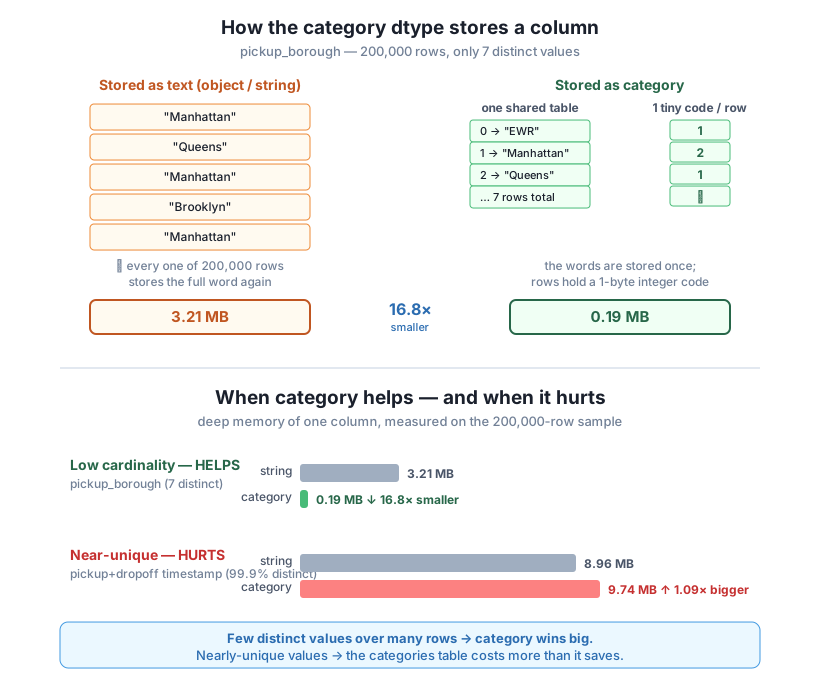
pickup_borough column from 3.21 MB as text to 0.19 MB — a 16.8x reduction, measured on the real taxi sample. Bottom: category helps enormously on a low-cardinality column (7 distinct values) but hurts on a near-unique column (99.9% distinct), where the overhead of holding almost 200,000 categories makes it 1.09x larger than plain text. Cardinality, not dtype, decides the outcome.If you also join the finer-grained Zone name (about 260 distinct values instead of 7), category still wins comfortably — that column drops from roughly 4.7 MB as text to 0.4 MB, a 12x cut — because 260 distinct values is still tiny next to 200,000 rows. The win shrinks a little as the number of categories grows, which is the clue to when it disappears entirely.
Category is not free magic. Its saving comes from one bet: there are far fewer distinct values than rows. When that bet is wrong — when nearly every value is unique — the categories table has to hold almost as many entries as there are rows, and you still pay for a code on every row. You end up storing everything twice.
To see it, build a column that is nearly unique. Concatenating each trip’s pickup and dropoff timestamps produces a near-unique “trip fingerprint” — almost no two trips share both. Now the category dtype has nothing to consolidate:
import warnings
warnings.filterwarnings("ignore")
import pandas as pd

CSV = "yellow_tripdata_sample.csv"

taxi = pd.read_csv(CSV)
trip_id = taxi["tpep_pickup_datetime"] + "_" + taxi["tpep_dropoff_datetime"]
print("rows:            ", len(trip_id))
print("distinct values: ", trip_id.nunique(),
      f"({100 * trip_id.nunique() / len(trip_id):.1f}% unique)")
mem_str = trip_id.memory_usage(index=False, deep=True)
mem_cat = trip_id.astype("category").memory_usage(index=False, deep=True)
print(f"as text:     {mem_str:>10,} bytes  ({mem_str/1024/1024:5.2f} MB)")
print(f"as category: {mem_cat:>10,} bytes  ({mem_cat/1024/1024:5.2f} MB)")
print(f"category is {mem_cat / mem_str:.2f}x the size of plain text -- it got BIGGER")
rows: 200000
distinct values: 199848 (99.9% unique)
as text: 9,400,000 bytes ( 8.96 MB)
as category: 10,217,837 bytes ( 9.74 MB)
category is 1.09x the size of plain text -- it got BIGGERWith 99.9% of the values distinct, converting to category added memory: 8.96 MB became 9.74 MB. The categories table now holds nearly 200,000 long strings — essentially the whole column over again — and on top of that pandas stores an int32 code for every row, because a single byte cannot address that many categories. You paid for the lookup machinery and got no consolidation in return.
This is the rule to remember: category pays off in proportion to how much values repeat. Low cardinality (a handful of values over many rows) is a big win. High cardinality (near-unique values) is a loss. A quick sanity check before converting any column is its cardinality ratio — col.nunique() / len(col). Close to 0 means convert with confidence; close to 1 means leave it as text.
A rule of thumb, not a hard line
There is no exact cardinality percentage where category flips from help to hurt — it depends on how long the repeated values are and how many rows you have. Long strings (borough names, city names, product titles) repeating even a few thousand times still favor category, because each avoided copy saves a lot of characters. The safe habit is to measure: convert the column, compare memory_usage(deep=True) before and after, and keep the change only if it actually shrank. You already have every tool you need to check.
Memory is the headline benefit, but categoricals also affect grouping — in one helpful way and one surprising way. The helpful way: grouping on a category column can be faster than grouping on the equivalent text column, because pandas groups on the compact integer codes instead of comparing strings. On the borough column:
import warnings
warnings.filterwarnings("ignore")
import pandas as pd
import time

CSV = "yellow_tripdata_sample.csv"
ZONES = "taxi_zone_lookup.csv"

taxi = pd.read_csv(CSV)
zones = pd.read_csv(ZONES)
pu = zones[["LocationID", "Borough"]].rename(
    columns={"LocationID": "PULocationID", "Borough": "pickup_borough"})
taxi = taxi.merge(pu, on="PULocationID", how="left")

as_text = pd.DataFrame({"borough": taxi["pickup_borough"].astype(str),
                        "fare": taxi["fare_amount"]})
as_cats = pd.DataFrame({"borough": taxi["pickup_borough"].astype("category"),
                        "fare": taxi["fare_amount"]})

def best_ms(df):
    best = float("inf")
    for _ in range(30):
        start = time.perf_counter()
        df.groupby("borough", observed=True)["fare"].mean()
        best = min(best, time.perf_counter() - start)
    return best * 1000

print(f"group-by on a text column:     {best_ms(as_text):.1f} ms")
print(f"group-by on a category column: {best_ms(as_cats):.1f} ms")
group-by on a text column: 4.9 ms
group-by on a category column: 3.6 msGrouping on the category column was faster — roughly 3.6 ms versus 4.9 ms here (the exact milliseconds vary from run to run and machine to machine, but the categorical is reliably quicker). On 200,000 rows the gap is small; on the full 2.96-million-row month it grows, which is exactly the kind of scaling CityFlow cares about.
Now the surprising way, and the one that bites people. By default, a group-by over a categorical produces a row for every category — even categories that never appear in the data. Group by two borough categoricals at once and pandas will, by default, generate every possible pair:
import warnings
warnings.filterwarnings("ignore")
import pandas as pd

CSV = "yellow_tripdata_sample.csv"
ZONES = "taxi_zone_lookup.csv"

taxi = pd.read_csv(CSV)
zones = pd.read_csv(ZONES)
pu = zones[["LocationID", "Borough"]].rename(
    columns={"LocationID": "PULocationID", "Borough": "pickup_borough"})
do = zones[["LocationID", "Borough"]].rename(
    columns={"LocationID": "DOLocationID", "Borough": "dropoff_borough"})
taxi = taxi.merge(pu, on="PULocationID", how="left").merge(do, on="DOLocationID", how="left")
taxi["pickup_borough"] = taxi["pickup_borough"].astype("category")
taxi["dropoff_borough"] = taxi["dropoff_borough"].astype("category")

n_cat = taxi["pickup_borough"].cat.categories.size
all_pairs = taxi.groupby(["pickup_borough", "dropoff_borough"], observed=False).size()
seen_pairs = taxi.groupby(["pickup_borough", "dropoff_borough"], observed=True).size()
print(f"borough categories: {n_cat}  ->  full grid = {n_cat} x {n_cat} = {n_cat**2} pairs")
print("observed=False rows:", len(all_pairs), "(every possible pair, even empty ones)")
print("observed=True  rows:", len(seen_pairs), "(only pairs that actually occur)")
borough categories: 7 -> full grid = 7 x 7 = 49 pairs
observed=False rows: 49 (every possible pair, even empty ones)
observed=True rows: 33 (only pairs that actually occur)With observed=False (still the historical default) pandas builds the full 7×7 grid of 49 pickup-dropoff combinations, filling the 16 pairs that never happened with empty groups. With observed=True you get only the 33 pairs that actually occur. On 7 boroughs the waste is trivial — 16 phantom rows. But group by two zone categoricals (260 × 260 ≈ 68,000 combinations) or three categoricals at once, and observed=False can explode into millions of empty groups and exhaust memory. The rule: whenever you group on categoricals, pass observed=True. Lesson 4 builds fast aggregations on top of this, and it always uses observed=True for exactly this reason.
Exercise 1 — Categorize the zone name and measure it. Load the taxi sample and the zone lookup, join on PULocationID to attach the Zone name (not the borough this time — the finer, ~260-value column), and print that column’s deep memory as text versus as a category, plus the reduction factor. Is the saving larger or smaller than the 16.8x you got for pickup_borough, and why?
Hint
Reuse the merge pattern from the lesson but rename Zone instead of Borough. Then compare col.memory_usage(index=False, deep=True) for col and col.astype("category"). Expect a big win but smaller than borough’s, because ~260 distinct values need a larger categories table than 7 — more categories means less consolidation.
Exercise 2 — Predict help or hurt with a cardinality ratio. Write a small function should_categorize(series) that returns the cardinality ratio series.nunique() / len(series) and a verdict string: "convert" if the ratio is below 0.5, "leave as-is" otherwise. Run it on payment_type, on the joined pickup_borough, and on the near-unique trip_id fingerprint from the lesson, and check the verdicts match what you measured.
Hint
The ratio is series.nunique() / len(series). For payment_type it is , essentially 0 → convert; for the near-unique fingerprint it is about 0.999 → leave as-is. Build the fingerprint with taxi["tpep_pickup_datetime"] + "_" + taxi["tpep_dropoff_datetime"]. A 0.5 cutoff is deliberately loose — the real decision is “measure if unsure,” but the ratio catches the obvious cases instantly.
Exercise 3 — Watch the codes get wider. Convert PULocationID (about 235 distinct zone IDs in the sample) to a category and print .cat.codes.dtype. Then convert the near-unique trip_id fingerprint to a category and print its .cat.codes.dtype. Explain why the two code dtypes differ, and connect that to why category helped one column and hurt the other.
Hint
With ~260 categories the codes fit in an int16 (up to about 32,000); with ~200,000 categories they need an int32. More distinct values force a wider code and a bigger categories table — the double cost that makes category lose on near-unique columns. payment_type, with 5 values, needed only an int8.
You learned how the category dtype trades a repeated value for a small integer code plus one shared table of the distinct values, and you measured exactly when that trade pays. On the real 200,000-row taxi sample, payment_type (5 distinct values) shrank 8x, from 1.6 MB to 200 KB, and a joined pickup_borough name column (7 distinct values, long strings) shrank 16.8x, from 3.21 MB to 0.19 MB. You then saw the honest limit: a near-unique trip fingerprint (99.9% distinct) got bigger as a category, 8.96 MB rising to 9.74 MB, because the categories table nearly duplicated the column and the codes widened to int32. Finally you previewed grouping: category group-bys run on compact codes and are a bit faster, but they default to materializing every category combination — so you always pass observed=True.
.cat.categories and .cat.codes expose the two pieces.payment_type, 16.8x on the text pickup_borough. The longer the repeated string and the fewer the distinct values, the bigger the win.int8 toward int32. Check nunique() / len() and measure before committing.observed=True on group-by — categorical group-bys otherwise materialize every possible category combination, which is harmless on 7 boroughs but catastrophic on multiple high-cardinality categoricals.CityFlow’s dashboard is built on readable labels — boroughs, zones, payment types — and those labels are the columns that repeat the most. Treating them as plain text quietly makes the taxi DataFrame several megabytes heavier than it needs to be, per label column, on every load. The category dtype turns those repeated labels into near-free columns, and on the full month the same 16.8x on a borough name is the difference between a join that fits in RAM and one that spills. Just as important, you learned to check first: category is a targeted tool, not a blanket “make it smaller” button, and pointing it at a near-unique column makes things worse. Measuring cardinality before converting is the habit that separates a reflex from an engineering decision.
You can now shrink the repeated-label columns that a taxi pipeline is full of, and you know how to tell a winning conversion from a wasteful one. Lesson 3, Efficient Operations & Copies, tackles a subtler drain: the memory that disappears not into fat dtypes but into duplicate DataFrames. Every time you write df2 = df[df["fare_amount"] > 0] or chain a series of transformations, pandas may quietly copy the whole frame — and two copies of a 400 MB DataFrame is 800 MB. You will learn when pandas copies versus when it returns a view, how to spot the SettingWithCopyWarning that signals an accidental copy, and how to transform columns in place so your carefully downcast, categorized taxi data stays lean instead of doubling behind your back.
Keep DATATWEETS free. Help fund practical data, AI, and engineering lessons for learners worldwide.

