Lesson 3 - Efficient Operations & Avoiding Copies

Welcome to Efficient Operations & Avoiding Copies#

CityFlow’s per-zone dashboard is coming together, but the pipeline that feeds it has a habit you can’t see from the outside: it keeps making copies. You read the taxi file, filter it, add a column, filter again, add another column, select the pieces you need — and every one of those steps quietly hands you a brand-new DataFrame while the previous one is still sitting in memory. On the 200,000-row teaching sample nobody notices. On a full month of nearly three million trips, that same pattern is exactly how a pipeline that “should” need half a gigabyte suddenly needs a gigabyte and a half and takes the kernel down with it.

The fix isn’t a magic flag. It’s understanding which pandas operations copy your data, and then writing your transformations so you never keep more copies alive than the work actually requires. In this lesson you’ll see filtering return a copy, watch the classic chained-indexing trap fail honestly under pandas 3.0’s Copy-on-Write rules, learn the single-.loc form that does what you meant, and finish by rebuilding a wasteful six-copy taxi pipeline as one lean method chain — measuring the real memory each one uses.

By the end of this lesson, you will be able to:

• Explain the difference between a view and a copy, and why filtering or selecting usually returns a copy that consumes its own memory.
• Recognize the chained-indexing trap and describe exactly what pandas 3.0’s Copy-on-Write does with it (a ChainedAssignmentError and no change to the original), then fix it with a single .loc call.
• Apply memory-saving habits: select columns before transforming, and avoid naming throwaway intermediate DataFrames.
• Rewrite a multi-copy pipeline as a method chain with .assign(), .query(), and .pipe(), and measure the peak-memory difference on real data.

Views versus copies#

Two DataFrames can relate to the same underlying data in one of two ways. A view is a window onto data that another object owns — change the view and the original changes too, because there is really only one array underneath. A copy owns its own separate data — change it and the original is untouched, because they no longer share anything. The distinction matters for memory because every copy is a second block of memory holding (some of) the same numbers.

The trouble is that it isn’t always obvious which one you got. Slicing, filtering with a boolean mask, and selecting columns can each return either, depending on the operation and the version of pandas. Start by loading CityFlow’s sample and filtering it, and inspect what came back:

# gate: skip
CSV = "https://datatweets.com/datasets/nyc-taxi/yellow_tripdata_sample.csv"

import warnings
import pandas as pd, numpy as np, tracemalloc

CSV = "yellow_tripdata_sample.csv"   # local copy of the sample above
trips = pd.read_csv(CSV, parse_dates=["tpep_pickup_datetime",
                                      "tpep_dropoff_datetime"])

print("rows:", f"{len(trips):,}")
print("columns:", trips.shape[1])
print("memory:", round(trips.memory_usage(deep=True).sum() / 1e6, 1), "MB")

rows: 200,000
columns: 10
memory: 16.0 MB

The full frame is 200,000 rows across 10 columns, about 16 MB. Now filter to the trips that actually charged a fare, and check whether the result shares memory with the original:

paid = trips[trips["fare_amount"] > 0]

print("filtered rows:", f"{len(paid):,}")
print("paid is a different object from trips:", paid is not trips)
print("paid owns its own data (not a view):",
      paid._mgr is not trips._mgr)

filtered rows: 197,321
paid is a different object from trips: True
paid owns its own data (not a view): True

Filtering with a boolean mask gave you a copy: paid is a distinct object with its own data manager, holding a fresh 197,321-row block of memory. That is usually what you want — but it means every filter in a pipeline is another allocation, and if you hold onto the intermediate frames, they all stay resident at once. When you deliberately want an independent copy, df.copy() makes it explicit; the danger is the copies you create by accident and never let go of.

The chained-indexing trap#

Here is the mistake that has confused pandas users for a decade. Suppose CityFlow decides that any trip recording zero passengers is a data-entry glitch and the count should be treated as 1. The instinct is to select those rows and assign to the column in one breath:

before = int((trips["passenger_count"] == 0).sum())

with warnings.catch_warnings(record=True) as caught:
    warnings.simplefilter("always")
    trips[trips["passenger_count"] == 0]["passenger_count"] = 1   # chained!

after = int((trips["passenger_count"] == 0).sum())

print("warning raised:", caught[0].category.__name__)
print("rows with passenger_count == 0 before:", before)
print("rows with passenger_count == 0 after: ", after)
print("did the change reach trips?", before != after)

warning raised: ChainedAssignmentError
rows with passenger_count == 0 before: 2154
rows with passenger_count == 0 after:  2154
did the change reach trips? False

Nothing changed. There were 2,154 zero-passenger rows before, and there are still 2,154 after. The assignment ran without an exception, but it silently did nothing to trips — and pandas warned you with a ChainedAssignmentError.

Why? Read trips[trips["passenger_count"] == 0]["passenger_count"] = 1 as two operations, because that is how Python executes it. First trips[trips["passenger_count"] == 0] runs and, as you just saw, produces a copy. Then ["passenger_count"] = 1 assigns into that copy. The copy is a temporary object with no name — the instant the line finishes, it’s discarded, taking your edit with it. Your original trips was never in the path.

The fix: one .loc, rows and column together#

The rule is: never index twice to assign. Do the row selection and the column selection in a single .loc[rows, column] call, so pandas sees one operation on one object and writes straight into trips:

trips.loc[trips["passenger_count"] == 0, "passenger_count"] = 1

print("rows with passenger_count == 0 now:",
      int((trips["passenger_count"] == 0).sum()))
print("mean passenger_count:", round(trips["passenger_count"].mean(), 3))

rows with passenger_count == 0 now: 0
mean passenger_count: 1.35

That worked: zero rows now hold a zero passenger count, and the column mean settled at 1.35. df.loc[mask, "col"] = value is the canonical, unambiguous way to update a subset of rows in place — one bracket, one operation, no throwaway copy in the middle. Whenever you catch yourself typing ][ in an assignment (something][...] =), stop: that second bracket is the trap.

Habit one: select columns before you transform#

Copies cost memory in proportion to how wide the frame is. So a cheap, reliable saving is to throw away the columns you don’t need before you start adding new ones, not after. Compare the two orders on the duration calculation:

def mb(df):
    return round(df.memory_usage(deep=True).sum() / 1e6, 1)

full = pd.read_csv(CSV, parse_dates=["tpep_pickup_datetime",
                                     "tpep_dropoff_datetime"])

# Wasteful: transform the whole 10-column frame, then narrow.
wide = full.copy()
wide["duration_min"] = ((wide["tpep_dropoff_datetime"]
                         - wide["tpep_pickup_datetime"])
                        / pd.Timedelta(minutes=1))

# Lean: keep only the 3 columns you need, then transform.
narrow = full[["PULocationID",
               "tpep_pickup_datetime",
               "tpep_dropoff_datetime"]].copy()
narrow["duration_min"] = ((narrow["tpep_dropoff_datetime"]
                           - narrow["tpep_pickup_datetime"])
                          / pd.Timedelta(minutes=1))

print("transform-then-narrow frame:", mb(wide), "MB")
print("narrow-then-transform frame:", mb(narrow), "MB")

transform-then-narrow frame: 17.6 MB
narrow-then-transform frame: 6.4 MB

Same duration column, same 200,000 rows, but the frame you carry through the transform is 6.4 MB instead of 17.6 MB — because the lean version stopped hauling seven columns it was never going to use. When this frame is one link in a longer chain of copies, that saving multiplies at every subsequent step. Reach for the columns you need up front; don’t compute over ballast.

Habit two: stop naming throwaway intermediates#

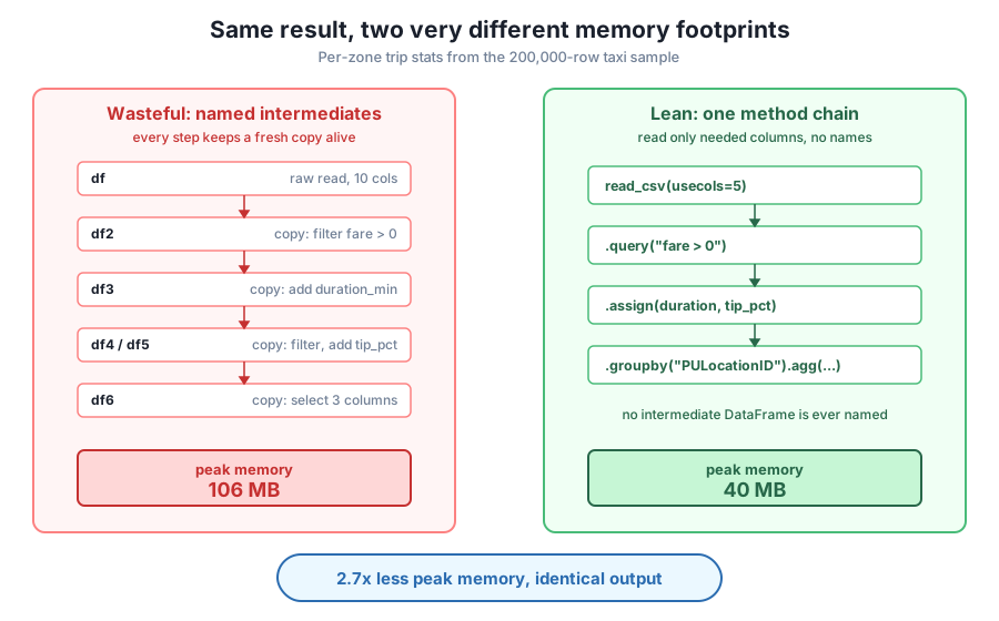
Now the main event. Here is a pipeline that computes CityFlow’s per-zone stats — trip count, average duration, average tip percentage — the way it often gets written first: one named DataFrame per step. It is easy to read line by line, and it is a memory sink, because df, df2, df3, df4, df5, and df6 all stay alive until the function returns. tracemalloc, Python’s built-in memory tracer, measures the real peak:

def wasteful():
    df  = pd.read_csv(CSV, parse_dates=["tpep_pickup_datetime",
                                        "tpep_dropoff_datetime"])
    df2 = df[df["fare_amount"] > 0]                     # copy: filter
    df3 = df2.copy()                                    # copy: explicit
    df3["duration_min"] = ((df3["tpep_dropoff_datetime"]
                            - df3["tpep_pickup_datetime"])
                           / pd.Timedelta(minutes=1))
    df4 = df3[df3["duration_min"] > 0]                  # copy: filter
    df5 = df4.copy()                                    # copy
    df5["tip_pct"] = df5["tip_amount"] / df5["fare_amount"] * 100
    df6 = df5[["PULocationID", "duration_min", "tip_pct"]]  # copy: select
    return (df6.groupby("PULocationID")
               .agg(trips=("duration_min", "size"),
                    avg_duration=("duration_min", "mean"),
                    avg_tip_pct=("tip_pct", "mean")))

tracemalloc.start()
wasteful_result = wasteful()
_, wasteful_peak = tracemalloc.get_traced_memory()
tracemalloc.stop()

print("wasteful peak memory:", round(wasteful_peak / 1e6, 1), "MB")
print("zones in result:", len(wasteful_result))

wasteful peak memory: 106.0 MB
zones in result: 235

Six named frames, and a peak of 106 MB to produce a tiny 235-row summary. Now rewrite it as a single method chain. Each method returns a new frame and passes it straight to the next call, so no intermediate ever gets a name — pandas is free to release each one the moment the next step consumes it. Two more wins are folded in: usecols reads only the five columns the pipeline touches, and .assign() and .query() keep the whole thing one flowing expression:

def lean():
    cols = ["tpep_pickup_datetime", "tpep_dropoff_datetime",
            "fare_amount", "tip_amount", "PULocationID"]
    return (
        pd.read_csv(CSV, usecols=cols,
                    parse_dates=["tpep_pickup_datetime",
                                 "tpep_dropoff_datetime"])
        .query("fare_amount > 0")
        .assign(
            duration_min=lambda d: ((d["tpep_dropoff_datetime"]
                                     - d["tpep_pickup_datetime"])
                                    / pd.Timedelta(minutes=1)),
            tip_pct=lambda d: d["tip_amount"] / d["fare_amount"] * 100,
        )
        .query("duration_min > 0")
        .groupby("PULocationID")
        .agg(trips=("duration_min", "size"),
             avg_duration=("duration_min", "mean"),
             avg_tip_pct=("tip_pct", "mean"))
    )

tracemalloc.start()
lean_result = lean()
_, lean_peak = tracemalloc.get_traced_memory()
tracemalloc.stop()

print("lean peak memory:", round(lean_peak / 1e6, 1), "MB")
print("same result as wasteful:",
      lean_result.round(6).equals(wasteful_result.round(6)))
print("memory ratio: {:.1f}x".format(wasteful_peak / lean_peak))

lean peak memory: 39.6 MB
same result as wasteful: True
memory ratio: 2.7x

Byte-for-byte the same 235-zone answer, at about 40 MB peak instead of 106 — about 2.7 times less memory. Nothing exotic did that. The chain just never held six full-width frames at once, and reading five columns instead of ten meant every step downstream was lighter too. The lambda d: ... inside .assign() is the key trick: it says “compute this new column from the frame at this point in the chain,” so you never need a variable to point at that frame.

.pipe() for steps that don’t fit a built-in method#

Sometimes a step in your chain is your own function — say, adding an average-speed column — and there’s no built-in method for it. .pipe(fn) slots any function that takes a DataFrame and returns one into the chain, so you don’t have to break the flow and name a variable just to call it:

def add_speed(d):
    hours = d["duration_min"] / 60
    return d.assign(speed_mph=np.where(hours > 0,
                                       d["trip_distance"] / hours,
                                       np.nan))

preview = (
    pd.read_csv(CSV, nrows=5,
                parse_dates=["tpep_pickup_datetime",
                             "tpep_dropoff_datetime"])
    .assign(duration_min=lambda d: ((d["tpep_dropoff_datetime"]
                                     - d["tpep_pickup_datetime"])
                                    / pd.Timedelta(minutes=1)))
    .pipe(add_speed)
)

print(preview[["trip_distance", "duration_min", "speed_mph"]]
      .round(2).to_string(index=False))

 trip_distance  duration_min  speed_mph
         17.14         31.92      32.22
          2.49         10.58      14.12
          1.84          6.82      16.20
          3.60         30.00       7.20
          0.04          1.57       1.53

add_speed reads like a stage in the pipeline rather than a detour: a 17-mile trip over 32 minutes clocks 32 mph (an airport run), while a 0.04-mile crawl manages 1.5 mph. .pipe() is what keeps method chaining from breaking down the moment your logic outgrows the built-in methods — your own transformations become links in the same chain.

Practice Exercises#

Exercise 1: Prove the chained-indexing trap, then fix it#

CityFlow wants every trip with trip_distance == 0 (a meterless glitch) recorded as a missing distance instead. First, reproduce the trap: capture warnings with warnings.catch_warnings(record=True) and run the chained form trips[trips["trip_distance"] == 0]["trip_distance"] = np.nan; print the warning’s class name and confirm, by counting zero-distance rows before and after, that nothing changed. Then do it correctly with a single .loc call and confirm the zero-distance count drops to 0.

Exercise 2: Measure a copy you didn’t mean to keep#

Load the sample into trips. Build a wasteful version that names three intermediates — step1 = trips[trips["fare_amount"] > 0], step2 = step1[step1["trip_distance"] > 0], step3 = step2[["PULocationID", "fare_amount", "trip_distance"]] — and wrap the three lines in tracemalloc to record the peak. Then build the same step3 result as a single method chain (.query(...).query(...)[[...]] or with .loc) and measure its peak. Print both peaks and confirm the two results are equal with .equals().

Exercise 3: Rebuild an aggregation as a lean chain#

Write a function zone_fares() that returns, per PULocationID, the trip count and the mean total_amount — but only for trips where fare_amount > 0 and passenger_count > 0. Write it as one method chain that (a) reads only the columns it needs with usecols, (b) filters with .query(), and (c) ends in .groupby("PULocationID").agg(...). No intermediate DataFrame should be named. Print the number of zones and the three zones with the highest mean total_amount.

Summary#

You saw where pandas spends memory you didn’t ask it to. Filtering trips returned a copy with its own 197,321-row block, not a view — and copies are how a pipeline’s footprint climbs. You reproduced the chained-indexing trap: trips[mask]["col"] = value assigns into a throwaway copy, and under pandas 3.0’s Copy-on-Write it raises a ChainedAssignmentError and leaves the original untouched (2,154 zero-passenger rows before and after). The correct single-.loc form fixed it in one operation. Then two habits — selecting columns before transforming (6.4 MB instead of 17.6), and threading a pipeline through one method chain instead of six named frames — cut a real per-zone aggregation from 106 MB to 40 MB peak, about 2.7x less, for a byte-identical 235-zone result.

Key Concepts#

• View vs copy. A view shares memory with another object; a copy owns its own. Filtering and column selection usually return a copy, so each one is a fresh allocation you’d rather not keep alive.
• .copy() is the explicit copy. Use it when you genuinely want independence; the memory problem is the accidental copies you hold onto.
• The chained-indexing trap. df[mask]["col"] = v writes into a temporary copy. In pandas 3.0 Copy-on-Write this raises ChainedAssignmentError and never reaches the original — reliably, on every machine, instead of the old undefined behavior.
• The fix is one .loc. df.loc[mask, "col"] = v selects rows and column in a single operation and writes in place.
• Select before you transform. Dropping unused columns up front shrinks every copy downstream.
• Method chaining with .query(), .assign(), and .pipe() avoids naming throwaway intermediates, so pandas can release each step — lower peak memory and code that reads like a recipe.

Why This Matters#

At 200,000 rows the difference between 106 MB and 40 MB is invisible; at 2.96 million rows it is the difference between a pipeline that runs and one that dies mid-aggregation on a machine that “should” have had enough RAM. Needless copies are among the most common reasons a pandas job uses far more memory than the data itself — and they hide in perfectly ordinary-looking code that names a new DataFrame at every step. Knowing which operations copy, refusing to hold intermediates you don’t need, and reaching for .loc instead of chained brackets are the habits that let the same transformation logic scale from a sample to a full month without a rewrite. They also make the correctness bug — the silently-dropped chained assignment — impossible, because you never write the pattern that causes it.

Continue Building Your Skills#

You can now spot the operations that copy your data and write transformations that don’t hoard them — the memory side of making pandas behave at scale. The pipelines here all ended in a groupby(...).agg(...), and so far you’ve taken that step for granted. In Lesson 4 you’ll turn your attention to the group-by itself: why a naive aggregation over millions of rows can be surprisingly slow, how the choice of aggregation functions and column dtypes changes its speed, and how to write group-bys that stay fast as CityFlow’s data grows from a sample to a full month. It’s the last core skill before the module’s guided project assembles downcasting, categoricals, copy-avoidance, and fast aggregation into one reusable, memory-measured taxi loader.