Title here
Summary here
Almost every tile on CityFlow’s dashboard is really a group-by in disguise. Revenue by payment type. Trips by hour of day. Average fare per pickup zone. Each one takes the millions of individual trips and collapses them into a small, readable table — a handful of numbers a stakeholder can actually look at. In pandas, the tool that does this is groupby(...).agg(...), and it is the single most-used move in analytics code.
Because you run it constantly, and because it touches every row, how you write a group-by decides whether a dashboard refresh takes a blink or a coffee break. In this lesson you’ll learn the fast, readable patterns on the real taxi sample: named aggregations that produce clean output columns, the one keyword — observed=True — that stops categorical group keys from exploding into tens of thousands of empty rows, and the habit of reaching for a built-in aggregation instead of a slow .apply(lambda ...). You’ll measure that last one and watch .agg() beat .apply() by about elevenfold for the exact same answer.
By the end of this lesson, you will be able to:
.agg(name=("column", "func"))) to get clean, well-labelled output columns.observed=True with categorical group keys to aggregate only the groups that actually exist, instead of the full Cartesian product..groupby().apply() is slow and replace it with a vectorized .agg(), measuring the speedup.transform to broadcast a per-group value (like a zone’s mean fare) back across every row.A group-by has three moving parts, always in the same order: split the rows into groups by some key, apply an aggregation to each group, and combine the results into one table with one row per group. When you write trips.groupby("payment_type").agg(...), pandas splits the 200,000 trips into buckets that share a payment type, computes your aggregation inside each bucket, and stacks the answers into a small result.
CityFlow’s reproducible teaching sample lives at https://datatweets.com/datasets/nyc-taxi/yellow_tripdata_sample.csv — 200,000 real trips, about 15 MB on disk:
# gate: skip
CSV = "https://datatweets.com/datasets/nyc-taxi/yellow_tripdata_sample.csv"
Load it, and add two helper columns the dashboard needs: a readable payment label (the raw payment_type is a numeric code, where 1 is a credit card and 2 is cash) and the hour of day each trip started, pulled straight off the pickup timestamp:
import warnings
warnings.filterwarnings("ignore")
import pandas as pd

CSV = "yellow_tripdata_sample.csv"   # local copy of the sample above
trips = pd.read_csv(CSV, parse_dates=["tpep_pickup_datetime",
                                      "tpep_dropoff_datetime"])

pay_labels = {1: "Credit card", 2: "Cash", 3: "No charge",
              4: "Dispute", 0: "Unknown"}
trips["pay"] = trips["payment_type"].map(pay_labels).fillna("Unknown")
trips["hour"] = trips["tpep_pickup_datetime"].dt.hour

print("rows:", f"{len(trips):,}")
rows: 200,000With the data loaded and two grouping keys ready, you can start collapsing 200,000 rows into dashboard-sized tables.
The readable way to aggregate is named aggregation: inside .agg(), you name each output column and say exactly which input column and function produce it, as output_name=("input_column", "function"). One .agg() call can build several columns at once, each with a name you chose — no cryptic total_amount_sum labels to rename afterward.
Here is CityFlow’s revenue-by-payment-type tile. For each payment method you want the trip count, the total revenue, the average fare, and the average tip — four aggregations, one call:
by_pay = (trips.groupby("pay")
          .agg(trips=("pay", "size"),
               revenue=("total_amount", "sum"),
               avg_fare=("fare_amount", "mean"),
               avg_tip=("tip_amount", "mean"))
          .sort_values("revenue", ascending=False))

print(by_pay.round(2))
trips revenue avg_fare avg_tip
pay
Credit card 156378 4415641.07 18.54 4.17
Cash 29522 668917.44 17.67 0.00
Unknown 9511 244642.50 19.98 1.52
No charge 1354 9958.03 5.34 0.02
Dispute 3235 4620.58 1.09 0.03One call, four clean columns, sorted by revenue. The story reads straight off the table: credit-card trips dominate, bringing in about million across 156,378 rides, while cash trips add another million. And notice the avg_tip column — cash trips average a $0.00 recorded tip, because cash tips are handed over in person and never make it into the data. That is not a bug; it is a real, well-known quirk of this dataset, and it is exactly the kind of thing a group-by surfaces in one glance.
The size function counts rows in each group (including any missing values), which is why trips=("pay", "size") gives the group’s headcount. Swap it for "sum", "mean", "min", "max", "median", "nunique", or "std" and you have covered most of what a dashboard ever asks for.
The same pattern answers the trips by hour of day tile — group by the hour column instead:
by_hour = (trips.groupby("hour")
           .agg(trips=("hour", "size"),
                avg_fare=("fare_amount", "mean"))
           .round(2))

print(by_hour.head(6))
print("busiest hour:", by_hour["trips"].idxmax(),
      "with", f"{by_hour['trips'].max():,}", "trips")
trips avg_fare
hour
0 5379 19.16
1 3626 17.29
2 2480 16.23
3 1654 17.47
4 1141 22.03
5 1322 28.16
busiest hour: 18 with 14,173 tripsThe pre-dawn hours are the quietest — the 4 a.m. hour sees just 1,141 trips — and the evening rush at 6 p.m. is busiest with 14,173. Same three-line pattern, a different key, another dashboard tile filled.
Aggregate the column you mean, not the whole frame
Named aggregation is precise on purpose: you spell out which column each result comes from. That saves you from the older style of calling .agg(["sum", "mean"]) on a whole grouped frame, which computes every function for every numeric column and hands back a wide, multi-level table you then have to dig through. Naming the two or three numbers you actually want keeps the output small and the code self-documenting — a reader sees revenue=("total_amount", "sum") and knows exactly what revenue is.
observed=True: don’t aggregate groups that don’t existIn the previous lesson’s module you learned to convert low-cardinality columns to the categorical dtype to save memory. Grouping by a categorical is fast — but it comes with a sharp edge that can silently blow up your results, and the fix is a single keyword.
When you group by two or more categorical columns, pandas defaults to producing a row for every possible combination of their categories — the full Cartesian product — even for combinations that never occur in the data. Watch what happens when CityFlow tries to build a pickup-zone by drop-off-zone trip matrix, with both location columns as categoricals:
trips["pay"] = trips["pay"].astype("category")
trips["PU"] = trips["PULocationID"].astype("category")
trips["DO"] = trips["DOLocationID"].astype("category")

n_pu = trips["PU"].cat.categories.size
n_do = trips["DO"].cat.categories.size
print("PU zones:", n_pu, " DO zones:", n_do,
      " possible pairs:", f"{n_pu * n_do:,}")

g_off = trips.groupby(["PU", "DO"], observed=False).agg(trips=("pay", "size"))
g_on  = trips.groupby(["PU", "DO"], observed=True ).agg(trips=("pay", "size"))

print("observed=False rows:", f"{len(g_off):,}")
print("observed=True  rows:", f"{len(g_on):,}")
print("empty groups created:", f"{len(g_off) - len(g_on):,}")
print("rows where trips == 0:", f"{(g_off['trips'] == 0).sum():,}")
PU zones: 235 DO zones: 251 possible pairs: 58,985
observed=False rows: 58,985
observed=True rows: 9,371
empty groups created: 49,614
rows where trips == 0: 49,614With observed=False (the historical default), pandas materialized all 58,985 zone pairs — every pickup zone crossed with every drop-off zone — even though only 9,371 of those routes were ever actually driven. That is 49,614 phantom rows, every one of them holding a trip count of zero, padding out your result table with combinations that never happened. Confirm the padding with memory:
mb_off = g_off.memory_usage(deep=True).sum() / 1e6
mb_on  = g_on.memory_usage(deep=True).sum() / 1e6
print(f"observed=False: {mb_off:.2f} MB")
print(f"observed=True:  {mb_on:.2f} MB")
observed=False: 0.71 MB
observed=True: 0.12 MBSetting observed=True aggregates only the groups that actually appear in the data, cutting this result from 58,985 rows to 9,371 and its memory from 0.71 MB to 0.12 MB. And this is the tame case: two location columns on a 200,000-row sample. Cross three or four high-cardinality categoricals and the empty combinations multiply until the “result” is far bigger than the data you started with — the classic way a categorical group-by exhausts memory and crashes.
Make observed=True your default for categorical group-bys
The rule is simple: whenever you group by one or more categorical columns, pass observed=True. With ordinary object or numeric keys the argument does nothing, because pandas only ever sees the values that are present. But the moment a key is categorical, observed=False invites the full Cartesian product of declared categories — including every combination that never occurred — and on multiple high-cardinality keys that is how a group-by explodes. You almost never want the empty combinations; when you genuinely do (say, to show a zero for every calendar month), reach for observed=False deliberately rather than inheriting it by accident.
.apply() when a built-in aggregation existsThere is one more habit that separates a fast group-by from a slow one, and it is the most common performance mistake in pandas code: reaching for .apply(lambda g: ...) when a built-in aggregation would do the same job.
The problem is where the work runs. Built-in aggregations like "sum" and "mean" execute in compiled C, once, across all groups. But .apply() calls your Python function once per group — and with hundreds of groups, that per-group Python overhead adds up fast, exactly the “interpreter tax” you met with loops in the last module. It is a loop over groups wearing a method’s clothing.
Here are two ways to build the same per-zone summary — trips, revenue, and average fare for each of the 235 pickup zones. The .apply() version writes a lambda that assembles a Series for each group; the .agg() version names the same three outputs:
def summary_apply():
    return trips.groupby("PU", observed=True).apply(
        lambda g: pd.Series({
            "trips":    len(g),
            "revenue":  g["total_amount"].sum(),
            "avg_fare": g["fare_amount"].mean(),
        }))

def summary_agg():
    return trips.groupby("PU", observed=True).agg(
        trips=("total_amount", "size"),
        revenue=("total_amount", "sum"),
        avg_fare=("fare_amount", "mean"))

import numpy as np
a, b = summary_apply(), summary_agg()
print("revenue matches: ", np.allclose(a["revenue"].values,  b["revenue"].values))
print("avg_fare matches:", np.allclose(a["avg_fare"].values, b["avg_fare"].values))
revenue matches: True
avg_fare matches: TrueThe two produce identical numbers — np.allclose confirms it column by column. Now put them on a stopwatch:
from timeit import timeit

apply_ms = min(timeit(summary_apply, number=1) for _ in range(3)) * 1000
agg_ms   = min(timeit(summary_agg,   number=5) for _ in range(3)) / 5 * 1000

print(f".apply(lambda): {apply_ms:7.1f} ms")
print(f".agg(named):    {agg_ms:7.2f} ms")
print(f"speedup:        {apply_ms / agg_ms:7.0f}x faster")
.apply(lambda): 62.7 ms
.agg(named): 5.90 ms
speedup: 11x fasterSame answer, but .agg() finishes in about 6 ms against .apply()’s 63 ms — roughly 11 times faster. The gap is the Python-per-group overhead: .apply() ran your lambda 235 times through the interpreter, while .agg() pushed all three aggregations down into C. Scale from this 200,000-row sample to a full month of nearly three million trips and that 11x becomes the difference between a snappy refresh and a dashboard that visibly stalls.
Your exact multiple will vary — the lesson won’t
Timings depend on your machine, your pandas build, and how many groups you have, so you might measure 8x or 15x rather than exactly 11x. The order of magnitude is the point: when a built-in aggregation exists, prefer it to .apply(). Save .apply() for the genuinely custom logic that has no vectorized equivalent — and even then, expect it to be the slow part. If a lambda inside .apply() is only calling .sum(), .mean(), .size(), or .max(), there is a named aggregation waiting to replace it and run many times faster.
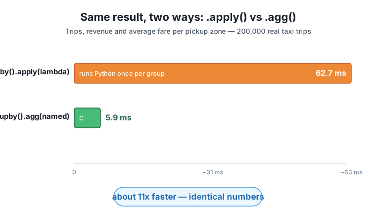
.groupby().apply(lambda) runs your Python function once for each of the 235 zone groups and takes about 62.7 ms; the equivalent .groupby().agg(named) pushes the sums and means into compiled C and takes about 5.9 ms — roughly 11x faster for byte-for-byte identical numbers. When a built-in aggregation exists, prefer it to .apply().transform: broadcast a per-group value back to every rowagg collapses each group to a single row. Sometimes you want the opposite: a per-group number pasted back onto every original row, so the result lines up with the input frame. That is what transform does.
CityFlow wants to know how each trip’s fare compares to the typical fare for its pickup zone — is this a pricier-than-usual ride, or a cheap one? You need each zone’s mean fare attached to every trip in that zone, then subtracted. transform("mean") computes the group mean and broadcasts it back to the same shape as the input, so it drops straight into a new column:
trips["zone_avg_fare"] = (trips.groupby("PU", observed=True)["fare_amount"]
                          .transform("mean"))
trips["fare_vs_zone"] = trips["fare_amount"] - trips["zone_avg_fare"]

print("result length matches input:",
      len(trips["fare_vs_zone"]) == len(trips))
print(trips[["PULocationID", "fare_amount", "zone_avg_fare", "fare_vs_zone"]]
      .head(5).round(2).to_string(index=False))
result length matches input: True
PULocationID fare_amount zone_avg_fare fare_vs_zone
132 70.0 59.48 10.52
163 13.5 14.86 -1.36
127 10.0 28.68 -18.68
186 23.3 15.84 7.46
238 3.7 13.41 -9.71Where agg would have returned one row per zone, transform returned 200,000 rows — one per trip — each carrying its own zone’s average fare. The first trip paid $70 in a zone that averages $59.48, so it was about $10.52 pricier than typical; the third paid $10 in a zone that averages $28.68, running nearly $19 below its zone’s norm. That “value minus its group mean” pattern — centring each row against its group — is the everyday use of transform, and it is just as vectorized as agg: no loop, one pass.
The quick way to remember which to use: agg when you want one row per group (a summary table), transform when you want a new column aligned to the original rows (a per-row comparison against the group).
Group the trips frame by passenger_count and, in a single .agg() call, build three named columns: trips (the row count in each group, using "size"), avg_distance (the mean of trip_distance), and avg_total (the mean of total_amount). Sort the result by trips in descending order and print it rounded to two decimals. Which passenger count is most common?
Hint
The pattern is trips.groupby("passenger_count").agg(trips=("passenger_count", "size"), avg_distance=("trip_distance", "mean"), avg_total=("total_amount", "mean")). Chain .sort_values("trips", ascending=False) and .round(2). You’ll see solo riders dominate — real taxi data is overwhelmingly one-passenger trips.
observed=TrueMake sure both trips["pay"] and a new categorical trips["hour_cat"] = trips["hour"].astype("category") are categorical, then group by both keys and count trips (.agg(n=("pay", "size"))) twice — once with observed=False and once with observed=True. Print the number of rows each produces and the difference. Explain in a sentence why the two differ.
Hint
With five payment labels and 24 hours, observed=False will try to make up to rows — every pay/hour pair, whether or not it occurred — while observed=True keeps only the pairs that actually appear. Compare len(...) of each result; the difference is the count of pay/hour combinations that never happened in the sample.
.apply() with a transformSuppose a teammate wrote trips.groupby("PU", observed=True)["tip_amount"].apply(lambda s: s - s.mean()) to compute each trip’s tip relative to its zone’s average tip. Rewrite it using transform instead so it runs faster, assign the result to a new tip_vs_zone column, and confirm the new column has the same length as trips. Print the five trips with the largest positive tip_vs_zone (the most generous tippers relative to their zone).
Hint
transform("mean") gives each row its zone’s mean tip; subtract it: trips["tip_vs_zone"] = trips["tip_amount"] - trips.groupby("PU", observed=True)["tip_amount"].transform("mean"). Use trips.nlargest(5, "tip_vs_zone") to see the top five. This does the same math as the .apply() version but keeps the work in compiled C.
You made group-by — the workhorse of every dashboard — both readable and fast on 200,000 real taxi trips. Named aggregations turned four numbers per payment type into one clean .agg() call, revealing that credit-card trips bring in about million and that cash trips record a $0.00 average tip. observed=True stopped a categorical zone-by-zone group-by from materializing 58,985 rows when only 9,371 routes exist, trimming 49,614 empty combinations and cutting memory from 0.71 MB to 0.12 MB. Swapping a .groupby().apply(lambda) for a vectorized .agg() produced identical numbers about 11x faster (63 ms down to 6 ms). And transform broadcast each zone’s mean fare back onto all 200,000 rows so you could centre every trip against its group.
.agg(name=("column", "func")) builds several cleanly-labelled output columns in one call; "size" counts rows, and "sum"/"mean"/"max"/"nunique" cover most needs.observed=True — with categorical group keys, aggregate only the combinations that actually occur; the default observed=False produces the full Cartesian product of categories, padding the result with empty groups (here 49,614 of them)..apply() when a built-in aggregation exists — .apply(lambda ...) runs Python once per group; the equivalent .agg() runs in compiled C and was about 11x faster for identical output.agg vs transform — agg returns one row per group (a summary); transform broadcasts a per-group value back to every original row (a per-row comparison), keeping the result aligned to the input.Group-by is where analytics code actually spends its time: every “by category”, “per zone”, “by hour” tile is a group-by over millions of rows, run again on every refresh. The three habits in this lesson — name your aggregations, pass observed=True on categorical keys, and prefer a built-in .agg() to a hand-written .apply() — are what keep those refreshes fast and their memory bounded as CityFlow’s data grows from a 200,000-row sample to full months of nearly three million trips. A .apply() that costs 11x more, or a categorical group-by that quietly balloons into tens of thousands of empty rows, is the kind of thing that works fine in testing and then stalls or crashes in production. Writing the fast version by default is a small habit that pays off every single time the pipeline runs.
You can now aggregate millions of rows into dashboard-sized tables quickly, without exploding memory on categorical keys or paying the .apply() tax. That completes the core pandas-at-scale toolkit: downcasting, categoricals, copy-aware transforms, and now fast group-by. In Lesson 5, the module’s guided project, you’ll assemble all of it into a single reusable memory-efficient taxi loader — a load_taxi() function that reads the raw data, downcasts numerics, converts low-cardinality columns to categoricals, and hands back a lean DataFrame — then measure the real memory it saves against a naive read_csv. Everything you’ve practised in this module comes together into one piece of production-ready code.
Keep DATATWEETS free. Help fund practical data, AI, and engineering lessons for learners worldwide.

