Lesson 5 - Guided Project: A Memory-Efficient Taxi Loader

Welcome to the Guided Project#

Across this module you have collected memory-saving techniques one at a time: downcasting numeric columns to the smallest safe type, converting low-cardinality columns to categoricals, avoiding the silent copies that double your memory, and writing group-by aggregations that stay fast on millions of rows. And back in Module 1 you wrote a reduction plan — a short, evidence-backed document that said exactly which columns to keep, which dtypes to change, and what the memory should be afterward. This project is where that plan stops being a document and becomes code.

You are still a data engineer at CityFlow. Every stage of the taxi pipeline starts the same way — some script reads a month of trips off disk — and right now each one loads the data naively, paying the full memory cost every time. Your deliverable is a single reusable function, load_taxi(), that reads a month of trips lean: only the columns the dashboard needs, each at the smallest dtype that still holds every real value, with the low-cardinality columns stored as categoricals. Write it once, import it everywhere, and every job in the pipeline gets the memory win for free.

You will work the full month — 2,964,624 real trips — not a sample, because the whole point is to measure the win at real scale. Every number below is measured, and you will reproduce every one of them.

By the end of this project, you will be able to:

• Measure the memory cost of a naive full-month load as an honest baseline
• Package the whole reduction plan — column selection, downcasting, and categoricals — into one reusable load_taxi() function
• Measure the real before-and-after memory and report the reduction as a factor and a percentage
• Confirm the lean load is loss-free by checking row counts and spot-checking values against the naive load
• Run a real analysis on the lean frame to prove it does full-scale work at a fraction of the memory

The dataset#

Everything runs on New York City’s public-domain Yellow Taxi trip records, published by the NYC Taxi & Limousine Commission (TLC). This project uses the full month — the official TLC Parquet file — because a memory win only means something measured at real scale:

• Full month, 2,964,624 rows, 19 columns: https://d37ci6vzurychx.cloudfront.net/trip-data/yellow_tripdata_2024-01.parquet

CityFlow also mirrors a smaller 200,000-row teaching sample for quick experiments, which you met earlier in the course:

• Teaching sample (10 columns): https://datatweets.com/datasets/nyc-taxi/yellow_tripdata_sample.csv

# gate: skip
FULL_MONTH = "https://d37ci6vzurychx.cloudfront.net/trip-data/yellow_tripdata_2024-01.parquet"
SAMPLE     = "https://datatweets.com/datasets/nyc-taxi/yellow_tripdata_sample.csv"

The code below downloads the full month once and then reads the local copy, exactly as a real pipeline caches a remote source file.

Stage 1: The naive baseline#

You cannot claim a saving without a number to save from, so the first job is to load the month the way an unsuspecting script would — read the whole Parquet file, take every column, accept pandas’ default dtypes — and measure what that costs in memory. This is the baseline every later number is compared against.

import warnings
warnings.filterwarnings("ignore")
import os
import urllib.request
import pandas as pd

# The full month of real NYC Yellow Taxi trips (public-domain TLC data).
url  = "https://d37ci6vzurychx.cloudfront.net/trip-data/yellow_tripdata_2024-01.parquet"
path = "yellow_tripdata_2024-01.parquet"
if not os.path.exists(path):
    urllib.request.urlretrieve(url, path)

naive = pd.read_parquet(path)
naive_mb = naive.memory_usage(deep=True).sum() / 1024**2

print(f"rows:         {len(naive):,}")
print(f"columns:      {naive.shape[1]}")
print(f"naive memory: {naive_mb:.1f} MB")

rows:         2,964,624
columns:      19
naive memory: 398.6 MB

There is the baseline: a naive load of the month holds all 19 columns and costs 398.6 MB in memory. Notice memory_usage(deep=True) — the deep=True counts the actual characters in text columns rather than just their pointers, so the total is the honest one. This 398.6 MB is the exact figure the reduction plan promised to attack, and it is the wall your load_taxi() has to get under.

Stage 2: Build load_taxi()#

Now package the plan. Rather than sprinkling astype calls through every script that touches the data, you write the reduction once as a function that reads a lean frame from the start. It combines four ideas from this module, in the order they apply:

1. Keep only the columns you need (columns=). The dashboard uses ten of the nineteen columns; the other nine — surcharges, flags, rate codes — never enter memory when you name the ten you want. This is the biggest single lever, and it happens at read time.
2. Downcast the integers (Lesson 1, with the ranges from Module 2). PULocationID and DOLocationID are zone IDs from 1 to 265, which fit in an int16 (up to 32,767) at a quarter of an int64’s size.
3. Downcast the floats. trip_distance and the three money columns are float64 by default but hold values with nowhere near enough significant digits to need 64 bits, so float32 halves each of them.
4. Categoricalize the low-cardinality column (Lesson 2). payment_type holds a handful of repeated codes that behave like labels, not numbers — a perfect categorical.

One column needs an honest judgement call. passenger_count looks like a small integer you could squeeze into an int8, but the real data has missing values in it, and pandas cannot store a NaN in an integer column. Forcing an integer type would either crash or silently invent a passenger count where there was none, so passenger_count stays a float — downcast to float32, the smallest float that still represents the missing marker. Letting the data, not the wish, decide the dtype is the whole discipline.

KEEP = [
    "tpep_pickup_datetime", "tpep_dropoff_datetime", "passenger_count",
    "trip_distance", "PULocationID", "DOLocationID", "payment_type",
    "fare_amount", "tip_amount", "total_amount",
]

def load_taxi(path, columns=KEEP):
    """Load the taxi parquet lean: only the needed columns, smallest safe dtypes."""
    df = pd.read_parquet(path, columns=columns)            # keep 10 columns, drop 9
    df = df.astype({
        "PULocationID":    "int16",    # zone IDs 1..265 fit in int16
        "DOLocationID":    "int16",
        "passenger_count": "float32",  # has missing values -> must stay float
        "trip_distance":   "float32",  # miles: 32-bit precision is plenty
        "fare_amount":     "float32",  # dollars
        "tip_amount":      "float32",
        "total_amount":    "float32",
    })
    df["payment_type"] = df["payment_type"].astype("int8").astype("category")
    return df

lean = load_taxi(path)
print(lean.dtypes.to_string())

tpep_pickup_datetime     datetime64[us]
tpep_dropoff_datetime    datetime64[us]
passenger_count                 float32
trip_distance                   float32
PULocationID                      int16
DOLocationID                      int16
payment_type                   category
fare_amount                     float32
tip_amount                      float32
total_amount                    float32

Every dtype is now the deliberate one, not the default. The two datetime columns are left as datetime64 — parsed straight from Parquet, they are already the native date type, and unlike the numbers they cannot be shrunk without throwing away resolution. Everything else is at its minimum: int16 zone IDs, float32 measurements and money, and payment_type as a category. The function takes a path and an optional columns list, so the same load_taxi() works for February, for March, or for a run that needs a different column set — write it once, reuse it forever.

Stage 3: Measure the win#

The function exists; now prove it earns its keep. Load the same month with load_taxi(), measure its memory, and compare it to the 398.6 MB baseline. A plan whose saving you have not measured is only a hope, so put a real number on it — and then, just as important, confirm you did not lose anything to get it.

lean_mb = lean.memory_usage(deep=True).sum() / 1024**2

print(f"naive load:  {naive_mb:6.1f} MB")
print(f"load_taxi(): {lean_mb:6.1f} MB")
print(f"reduction:   {naive_mb/lean_mb:.2f}x  ({100*(1 - lean_mb/naive_mb):.1f}% saved)")

print(f"rows kept:            {len(lean):,} of {len(naive):,}")
print(f"fare_amount sum naive: {naive['fare_amount'].sum():.2f}")
print(f"fare_amount sum lean:  {lean['fare_amount'].astype('float64').sum():.2f}")
print("PULocationID identical:", (naive['PULocationID'].astype('int16') == lean['PULocationID']).all())

naive load:   398.6 MB
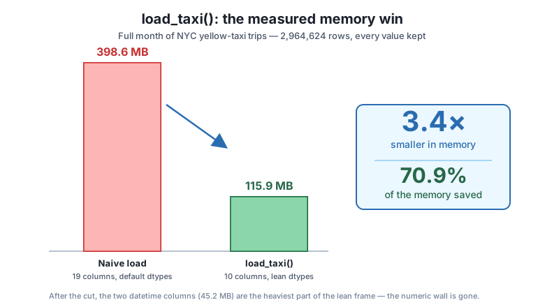
load_taxi():  115.9 MB
reduction:   3.44x  (70.9% saved)
rows kept:            2,964,624 of 2,964,624
fare_amount sum naive: 53882224.76
fare_amount sum lean:  53882224.79
PULocationID identical: True

The plan holds up at full scale. The naive 398.6 MB load becomes 115.9 MB through load_taxi() — a 3.44x reduction, 70.9% of the memory gone — and every one of the 2,964,624 rows is still there. The integrity checks confirm the data survived the shrink: the PULocationID values are identical after the int16 downcast (zone IDs are small integers, so nothing is lost), and the fare_amount totals agree to the penny in the millions (53,882,224.76 vs 53,882,224.79). That last tiny gap is the honest signature of float32: it carries about seven significant digits, so summing three million dollar amounts drifts by a few cents in the eighth digit — invisible for a dashboard, and the reason float32 is the right trade for money at this scale rather than a lossy shortcut.

Where did the 115.9 MB end up? Break the lean frame down column by column to see what is left:

print((lean.memory_usage(deep=True).drop("Index") / 1024**2).round(2).to_string())

tpep_pickup_datetime     22.62
tpep_dropoff_datetime    22.62
passenger_count          11.31
trip_distance            11.31
PULocationID              5.65
DOLocationID              5.65
payment_type              2.83
fare_amount              11.31
tip_amount               11.31
total_amount             11.31

The wall of identical 22.62 MB columns from the naive profile is gone. The float32 columns now cost 11.31 MB apiece (exactly half their old width), the int16 zone IDs just 5.65 MB, and payment_type a mere 2.83 MB as a categorical. What remains at the top are the two datetime64 columns at 22.62 MB each — together 45.2 MB, now the single heaviest part of the frame precisely because they are the one thing you could not shrink. That is the tell-tale sign of a well-reduced DataFrame: the leftover cost sits in the columns that genuinely need their bytes.

Stage 4: Use it#

A lean loader is only worth building if the lean frame does real work, so put it to the test. The dashboard needs a revenue breakdown by payment type — how many trips each method carried, how much money it brought in, and the average fare and tip on it. This is a group-by aggregation over all 2.96 million rows, run on the frame that costs a third of the naive memory, and grouping on the categorical payment_type is exactly the fast path the categorical was chosen for.

labels = {0: "Unknown", 1: "Credit card", 2: "Cash", 3: "No charge", 4: "Dispute"}
by_pay = lean.groupby("payment_type", observed=True).agg(
    trips=("total_amount", "size"),
    revenue=("total_amount", "sum"),
    avg_fare=("fare_amount", "mean"),
    avg_tip=("tip_amount", "mean"),
).sort_values("revenue", ascending=False)

print(f"{'payment_type':>16}{'trips':>12}{'revenue_$M':>13}{'avg_fare':>10}{'avg_tip':>9}")
for pt, row in by_pay.iterrows():
    name = f"{int(pt)} {labels.get(int(pt), '?')}"
    print(f"{name:>16}{int(row.trips):>12,}{row.revenue/1e6:>13.2f}"
          f"{row.avg_fare:>10.2f}{row.avg_tip:>9.2f}")

total = lean["total_amount"].astype("float64").sum()
print(f"\nmonth revenue: ${total/1e6:.1f}M across {len(lean):,} trips")
print(f"credit-card share of revenue: {by_pay.loc[1, 'revenue'] / total * 100:.1f}%")

    payment_type       trips   revenue_$M  avg_fare  avg_tip
   1 Credit card   2,319,046        65.53     18.56     4.17
          2 Cash     439,191        10.05     17.87     0.00
       0 Unknown     140,162         3.62     20.02     1.55
     3 No charge      19,597         0.17      6.75     0.01
       4 Dispute      46,628         0.08      1.33     0.04

month revenue: $79.5M across 2,964,624 trips
credit-card share of revenue: 82.5%

The lean frame answers the real question without breaking a sweat. NYC yellow taxis booked $79.5 million across the month, and the breakdown is striking: credit cards carry 82.5% of the revenue (2.3 million trips) and, tellingly, the entire tip signal. Card riders tip $4.17 on average while cash trips record an average tip of $0.00 — not because cash riders never tip, but because cash tips are handed over outside the meter and simply never reach the data. That is a genuine insight for the dashboard and a caveat the team needs to state honestly: any “tipping” chart is really a chart of card tips. The small No charge and Dispute groups, with their tiny fares, are the adjustments and voided trips you flagged as dirty data back in Module 1 — visible here as the low-revenue tail.

Every one of those aggregates was computed on the 115.9 MB frame, not the 398.6 MB one. Same rows, same answer, a third of the RAM — which means three of these jobs can now run in the memory that one naive load used to hog. That is the entire payoff of the module, delivered by a single reusable function.

Practice Exercises#

These extend the loader you just built. The naive DataFrame (full month, 19 columns) and the lean frame from load_taxi() are both still in memory, along with the load_taxi function and the path.

Exercise 1. The dashboard team wants a borough-level view, which means keeping location IDs but adding the zone lookup later. First, quantify what the categorical bought you: reload payment_type as a plain int8 instead of a category and compare its memory to the 2.83 MB categorical version. Is the categorical actually smaller here, and if the difference is small, what other reason is there to prefer it?

Exercise 2. Make load_taxi() do a little more work. Add a computed trip_minutes column — the dropoff minus pickup, in minutes, as float32 — and then, because the two datetime columns are now the heaviest part of the frame, drop them and keep only trip_minutes. Measure the memory of this duration-only frame and compare it to the 115.9 MB version. How much did dropping the two 22.62 MB datetime columns for one 11.31 MB float column save?

Exercise 3. A teammate proposes downcasting the money columns all the way to float16 “to save even more.” Test whether that is safe: cast total_amount to float16, sum it, and compare the total to the float32 sum of $79.5 M. Explain in a comment why the numbers diverge and why float32, not float16, is the right floor for dollar amounts at this scale.

Summary#

You turned Module 1’s reduction plan into a single reusable function and measured the win on the real full month. A naive load of all 2,964,624 rows cost 398.6 MB; your load_taxi() — keeping only the ten dashboard columns, downcasting integers to int16 and floats to float32, and storing payment_type as a categorical — cut it to 115.9 MB, a measured 3.44x reduction (70.9% saved) with every row intact and values verified against the naive load. You saw that the leftover cost sits in the two datetime64 columns you deliberately could not shrink, and you handled the real dirty data honestly by keeping passenger_count as a float because it has missing values. Finally you ran a real revenue-by-payment-type analysis on the lean frame — $79.5 M for the month, 82.5% on credit cards, cash tips invisible in the data — proving the efficient loader does full-scale work at a third of the memory.

Key Concepts#

• A loader is the right place for the reduction plan — applying column selection, downcasting, and categoricals once inside load_taxi() means every job in the pipeline inherits the memory win instead of re-deriving it.
• Select columns at read time — passing columns= to read_parquet skips the unwanted columns on disk, which is cheaper than loading everything and dropping afterward.
• Downcast to the smallest dtype that still fits the real values — int16 for 1–265 zone IDs, float32 for measurements and money; the choice is measured against the data’s actual range, not guessed.
• Let the data veto a dtype — passenger_count stays a float because it has missing values that an integer column cannot hold; honesty about the data beats the smaller type.
• Measure the win and verify no loss — report the reduction as a factor and a percentage, and confirm row counts and spot-checked sums match the naive load before trusting the lean frame.

Why This Matters#

Every data pipeline reads its source data over and over — once per job, once per retry, once per developer poking at it locally — and a naive loader makes each of those reads pay full price. Folding the reduction plan into a single load_taxi() means the saving is applied consistently and automatically: the same 398.6 MB month that used to crowd a machine now fits three times over in the same RAM, so more jobs run in parallel, containers need less memory, and a laptop can hold data that used to demand a server. Just as important, you proved the win is free of cost to correctness — identical row counts, penny-accurate sums — so there is no trade-off to agonize over. This is the everyday craft of a data engineer: build the lean path once, measure that it loses nothing, and let every downstream job ride on it.

Continue Building Your Skills#

That completes Module 3: Pandas at Scale. You can now downcast numeric columns safely, reach for categoricals on low-cardinality data, transform frames without triggering wasteful copies, aggregate quickly with group-by, and — as of this project — package the whole reduction plan into a reusable load_taxi() that cuts a real month of taxi data by more than 3x while proving it loses nothing.

There is a ceiling to this approach, though, and you have just brushed against it: load_taxi() still holds the entire lean frame — 115.9 MB, or the whole 2.96-million-row month — in memory at once. That works comfortably for one month on a normal machine, but a full year of trips, or a dataset that is lean and still larger than your RAM, will not fit no matter how aggressively you downcast. Next comes Module 4: Chunked & Out-of-Core Processing, where you stop assuming the data fits at all. You will read the taxi file in bounded chunks, aggregate across those chunks without ever materializing the whole thing, and process data that is larger than memory using the same lean-dtype habits you built here — the natural next move once shrinking a DataFrame is no longer enough on its own.