Lesson 1 - Why Parallelism (and the GIL)

Welcome to Why Parallelism (and the GIL)#

Every pipeline you have built for CityFlow so far has been correct, memory-lean, and slow in one specific way: it used a single CPU core. Module 4 streamed a whole month of trips through iter_batches, aggregated per zone and day, and never loaded more than one batch at a time — a genuine achievement for memory, but while that code ran, a top reading would have shown one core pinned at 100% and the other nine sitting at roughly zero. On a 10-core machine, that is 90% of the hardware idle. Parallelism is the fix: doing independent pieces of work at the same time on multiple cores, so a job that takes ten seconds on one core can, in the best case, finish in closer to one.

The catch — and the reason this lesson exists before any of the how-to lessons — is that in Python the obvious tool for “do many things at once” does not speed up the work data engineers usually have. Reaching for threads on a CPU-bound Python job gives you almost nothing, because of a single design decision in CPython called the Global Interpreter Lock. So this lesson does two things: it draws the line between the work threads help and the work they don’t, and then it proves the line with a measurement you can reproduce — the same computation on six taxi partitions, run three ways, timed honestly. By the end you’ll understand exactly why the rest of this module is built on multiprocessing, not threads.

By the end of this lesson, you will be able to:

• Explain what parallelism buys a data pipeline, and why using one core wastes a modern machine
• Tell CPU-bound work apart from I/O-bound work, and predict which one threads can accelerate
• Describe what the Global Interpreter Lock (GIL) locks, and why it caps threaded CPU-bound Python at one core’s throughput
• Run the identical taxi computation serially, across threads, and across processes, and measure the speedup of each
• Explain why processes win where threads fail, and structure a gate-safe multiprocessing script

You’ll need pyarrow and Python’s standard library. Let’s put the whole machine to work.

One Core, Nine Idle#

Start by asking the machine how much parallelism is even on the table. The answer is the number of logical CPU cores it exposes:

import warnings
warnings.filterwarnings("ignore")
import os

if __name__ == "__main__":
    print("logical CPU cores available:", os.cpu_count())

logical CPU cores available: 10

Ten cores. Every serial pipeline so far has used exactly one of them at a time, which means the ceiling on how much faster this work could go is large — up to roughly 10x if the work divided perfectly, though we’ll see it never divides perfectly. The opportunity is real, but before we spend it we have to know which kind of work responds to more cores, because not all of it does.

CPU-Bound vs I/O-Bound#

Every step in a pipeline spends its time in one of two ways, and the difference decides whether more cores can help.

I/O-bound work spends most of its time waiting — for a disk to return bytes, for a network socket to deliver the next chunk of a download, for a database to answer a query. The CPU is largely idle during that wait; the bottleneck is the device, not the processor. Reading yellow_tripdata_2024-01.parquet off disk, downloading it from the TLC servers, or issuing a SELECT to the SQLite warehouse you built in Module 4 are all I/O-bound.

CPU-bound work spends its time computing — the processor is busy the whole time and the answer comes faster only if the chip goes faster or you use more of it. Parsing two timestamp strings into datetime objects, subtracting them to get a trip duration, dividing distance by time to get miles per hour, and testing that against an anomaly threshold — done in a Python loop, once per trip, six million times — is CPU-bound. There is no waiting; every microsecond is arithmetic and object creation.

The taxi pipeline has both. Reading a row group is I/O; the per-trip math on the rows you read is CPU. This distinction is not academic, because the tool you would naturally reach for — threads — helps exactly one of them:

• For I/O-bound work, threads genuinely help. While one thread waits on the disk or network, Python hands the processor to another thread to do useful work. Ten threads each waiting on a slow download can overlap their waits and finish far sooner than one thread doing them one after another.
• For CPU-bound pure-Python work, threads do not help — and can even hurt. There is no wait to overlap; every thread wants the processor for real computation at the same moment, and Python will not let them have it. To understand why, you need to meet the lock.

What the GIL Actually Locks#

CPython — the standard Python interpreter you are almost certainly running — protects its internal state with a single mutex called the Global Interpreter Lock, or GIL. The rule it enforces is short and consequential: only one thread may execute Python bytecode at a time. A thread must hold the GIL to run Python instructions, and there is exactly one GIL per process, so no matter how many threads you start, their Python code runs one thread at a time, taking turns on a single core’s worth of execution.

This is why threads help I/O but not CPU work. When a thread makes a blocking I/O call — reading a file, waiting on a socket — CPython releases the GIL during the wait, letting another thread run Python in the meantime. The waiting costs no Python execution, so the turns overlap productively. But when six threads all want to run a tight Python compute loop, there is nothing to overlap: they queue for the one GIL, each running a little before handing it on, and the total Python throughput is that of a single core. You have paid for the overhead of coordinating six threads and received the performance of one. (NumPy and pandas soften this for vectorized work, because their C routines release the GIL while crunching arrays — but a per-row Python loop like our anomaly check runs pure Python bytecode, fully under the lock.)

The consequence for data engineering is stark, and rather than take it on faith we’ll measure it.

The Setup: Six Partitions, One Heavy Worker#

The unit of parallel work in this module is a row group — the natural partition inside a Parquet file. Each of CityFlow’s two months (January and February 2024) has three row groups of roughly a million trips, so Jan plus Feb gives six partitions, about six million trips total. That is the workload we’ll run three ways.

The two months come from the public TLC trip-record site. Fetch them once and save them next to your script; every runnable block below reads the local copies by name:

# gate: skip
# CityFlow's two months of yellow-taxi trips, fetched once from the public TLC site.
import urllib.request
base = "https://d37ci6vzurychx.cloudfront.net/trip-data/"
for name in ["yellow_tripdata_2024-01.parquet", "yellow_tripdata_2024-02.parquet"]:
    urllib.request.urlretrieve(base + name, name)

Now the worker. This is the heavy per-trip computation — deliberately written as a Python loop so the cost lands squarely on the interpreter, exactly the CPU-bound shape that exposes the GIL. Crucially, the worker takes a tiny (path, row_group_index) tuple and reads its own partition; it is never handed a big DataFrame. That keeps this pattern honest for parallelism (there is no giant object to serialize and ship to a worker — a cost Lesson 4 measures in detail) and it makes the function importable and picklable, which multiprocessing requires. Define it at the top level of your script:

import warnings
warnings.filterwarnings("ignore")
import time
import multiprocessing as mp
from concurrent.futures import ThreadPoolExecutor
from datetime import datetime
import pyarrow.parquet as pq

FILES = ["yellow_tripdata_2024-01.parquet", "yellow_tripdata_2024-02.parquet"]
COLUMNS = ["tpep_pickup_datetime", "tpep_dropoff_datetime", "trip_distance", "fare_amount"]

def heavy_partition(task):
    """Read ONE row group and do heavy per-trip Python work. task = (path, row_group_index)."""
    path, i = task
    tbl = pq.ParquetFile(path).read_row_group(i, columns=COLUMNS).to_pandas()
    trips = 0
    anomalies = 0
    for pick, drop, dist, fare in zip(
        tbl["tpep_pickup_datetime"].astype(str),
        tbl["tpep_dropoff_datetime"].astype(str),
        tbl["trip_distance"],
        tbl["fare_amount"],
    ):
        minutes = (datetime.fromisoformat(drop) - datetime.fromisoformat(pick)).total_seconds() / 60.0
        mph = dist / (minutes / 60.0) if minutes > 0 else 0.0
        if mph > 80 or minutes < 0 or fare < 0:
            anomalies += 1
        trips += 1
    return (trips, anomalies)

That block only defines things, so it prints nothing on its own. The next block builds the list of six tasks — one per row group — and shows them:

if __name__ == "__main__":
    tasks = [(f, i) for f in FILES for i in range(pq.ParquetFile(f).metadata.num_row_groups)]
    print("partitions to process:", len(tasks))
    for t in tasks:
        print("  ", t)

partitions to process: 6
   ('yellow_tripdata_2024-01.parquet', 0)
   ('yellow_tripdata_2024-01.parquet', 1)
   ('yellow_tripdata_2024-01.parquet', 2)
   ('yellow_tripdata_2024-02.parquet', 0)
   ('yellow_tripdata_2024-02.parquet', 1)
   ('yellow_tripdata_2024-02.parquet', 2)

Six independent tasks, each a small tuple. Nothing about the work forces them to run in sequence — that is the definition of embarrassingly parallel work, and it is the ideal case for what follows.

Run 1: Serial (the Baseline)#

First the honest baseline — process all six partitions one after another, on one core, and time it:

if __name__ == "__main__":
    start = time.perf_counter()
    serial_results = [heavy_partition(t) for t in tasks]
    serial_secs = time.perf_counter() - start
    total_trips = sum(r[0] for r in serial_results)
    total_anomalies = sum(r[1] for r in serial_results)
    print(f"serial:      {serial_secs:5.2f}s   trips={total_trips:,}   anomalies={total_anomalies:,}")

serial:       9.60s   trips=5,972,150   anomalies=80,206

Just under ten seconds to grind through 5,972,150 trips on one core, flagging 80,206 with an impossible speed or a negative duration or fare. This is the number every other run has to beat. (Exact seconds vary from machine to machine and run to run — yours will differ, but the ratios between the three runs are the point, and those hold.)

Run 2: Six Threads (the GIL Shows Up)#

Now hand the same six tasks to a pool of six threads and let them run “concurrently.” ThreadPoolExecutor.map applies heavy_partition to each task, spreading them across the six threads:

if __name__ == "__main__":
    start = time.perf_counter()
    with ThreadPoolExecutor(max_workers=6) as pool:
        thread_results = list(pool.map(heavy_partition, tasks))
    thread_secs = time.perf_counter() - start
    print(f"threads x6:  {thread_secs:5.2f}s   speedup vs serial = {serial_secs / thread_secs:.2f}x")

threads x6:   9.19s   speedup vs serial = 1.04x

Six threads, and the work finished at 1.04x — statistically indistinguishable from serial. This is the GIL, exactly as advertised. The six threads did overlap their brief file-reading waits, which is why it is a hair faster rather than slower, but the dominant cost is the per-trip Python loop, and that ran one thread at a time under the single GIL. Six workers, one core’s worth of Python throughput. (On a busy machine you may even see threads come out slower than serial, because the overhead of shuffling the GIL between six contending threads outweighs the tiny I/O overlap — threads are not a speedup here, they are at best a wash.)

Run 3: Six Processes (True Parallelism)#

Same tasks, same worker, one change: swap the thread pool for a multiprocessing.Pool of six processes.

if __name__ == "__main__":
    start = time.perf_counter()
    with mp.Pool(processes=6) as pool:
        process_results = pool.map(heavy_partition, tasks)
    process_secs = time.perf_counter() - start
    print(f"processes x6:{process_secs:5.2f}s   speedup vs serial = {serial_secs / process_secs:.2f}x")

processes x6: 2.42s   speedup vs serial = 3.96x

There it is — 2.42 seconds, a 3.96x speedup from the identical code that threads ran flat. Six processes did what six threads could not: run the CPU-bound Python loop genuinely at the same time. That is the entire lesson in three numbers, and the figure lines them up:

Why Processes Win Where Threads Fail#

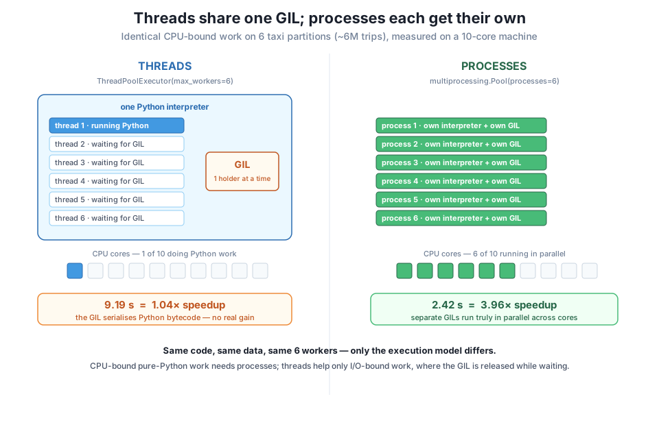
The mechanism is simple once the GIL is clear. A thread pool creates threads inside one process, so they share that process’s single interpreter and single GIL — and Python’s one-thread-at-a-time rule caps them at a single core’s throughput for pure-Python work. A process pool creates separate operating-system processes, and each process is a complete, independent Python runtime: its own memory, its own interpreter, and — the decisive part — its own GIL. Six GILs, six interpreters, six cores, all executing Python bytecode at the same instant. The lock that serialised the threads doesn’t exist between processes, because there is nothing shared for it to protect.

That independence is exactly why processes are slightly sublinear rather than a clean 6x: 3.96x, not 6.00x. Two forces hold it back. First, spinning up six fresh interpreters under spawn takes real time before any trip is processed. Second, the six row groups are not perfectly equal, so the pool waits for the slowest one to finish — the job is only as fast as its largest partition. Lesson 3 formalises this ceiling as Amdahl’s law; for now the honest headline is that processes turned a ten-second job into a two-and-a-half-second one, and threads did not move it at all.

The independence has a price, too, and it is the flip side of “no shared GIL”: no shared memory. Threads can read the same DataFrame in memory for free; processes cannot — anything a process needs must be sent to it, pickled and copied across a process boundary. This is precisely why heavy_partition takes a tiny (path, index) tuple and reads its own partition, instead of receiving a million-row DataFrame. Sending big objects to workers can cost more than the parallelism saves; Lesson 4 measures that trap directly. For this lesson the rule of thumb is enough: give workers small arguments and let them fetch their own data.

Practice Exercises#

Exercise 1 — Reproduce the three-way race on your machine. Using heavy_partition and the six-task list from this lesson, time the serial run, the ThreadPoolExecutor(max_workers=6) run, and the multiprocessing.Pool(processes=6) run, and print each one’s seconds together with its speedup versus serial. Your exact seconds will differ from the lesson’s, but confirm the shape: threads land near 1x while processes land well above it.

Exercise 2 — Show that trivial work does not parallelize. Write a second worker, light_partition(task), that reads the same row group but does only a fast vectorized reduction — for example return float(tbl["fare_amount"].mean()) — with no Python per-row loop. Run the six tasks serially and again with a six-process Pool, and compare the times. Explain in a comment why processes fail to win (and may lose) here even though they crushed the heavy version.

Exercise 3 — Watch the speedup curve bend. Run the heavy workload through a process pool with processes=2, then 4, then 6, timing each, and print the speedup versus serial for all three. You should see the speedup rise but sublinearly — nowhere near 2x, 4x, 6x. Note in a comment which of the six unequal partitions you think is setting the floor, and why more workers stop helping.

Summary#

You established why the rest of this module uses processes. Parallelism means running independent work at the same time across multiple cores, and a modern 10-core machine leaves most of its power unused when a pipeline runs serially. But more cores help only the right kind of work: I/O-bound work (waiting on disk, network, or a database) can be overlapped by threads because CPython releases the GIL during the wait, while CPU-bound pure-Python work (per-row parsing and math) cannot, because the Global Interpreter Lock allows only one thread to execute Python bytecode at a time. You proved it by running one heavy per-trip computation on six taxi partitions three ways: serial at 9.60 s, six threads at 9.19 s (1.04x — the GIL barely moves it), and a six-process Pool at 2.42 s (3.96x). Processes win because each carries its own interpreter and its own GIL and so runs truly in parallel; the price is no shared memory, which is why each worker takes a small (path, index) tuple and reads its own partition rather than receiving a pickled DataFrame.

Key Concepts#

• Parallelism vs one core — serial pipelines use a single core; a 10-core machine can, in principle, go much faster on independent work, but only work that is genuinely CPU-bound and divisible benefits.
• CPU-bound vs I/O-bound — I/O-bound work waits on a device and is helped by threads; CPU-bound pure-Python work keeps the processor busy and is not. Reading a file is I/O; the per-trip loop is CPU.
• The GIL — CPython’s Global Interpreter Lock lets only one thread run Python bytecode at a time, so N threads doing CPU-bound Python share one core’s throughput. The GIL is released during blocking I/O, which is why threads still help there.
• Processes each own a GIL — separate processes have independent interpreters and independent GILs, so they execute Python in genuine parallel; the trade-off is no shared memory, so data must be sent to them.
• Gate-safe structure — the worker lives at the top level (importable, picklable); all pool creation, timing, and printing live inside if __name__ == "__main__":, because spawn re-imports the script in every child. Run it as a .py script.

Why This Matters#

For CityFlow, this is the difference between a nightly aggregation that finishes before the dashboard refresh and one that misses it. The processing you built in Module 4 was correct but single-core; the same work spread across a process pool can run three to four times faster with no change to the logic — you just have to structure it so the workers are independent and cheap to feed. Equally important is the discipline the lesson models: never assume a parallelism strategy, measure it. The threaded run looked reasonable and delivered nothing; only the timings exposed the GIL. Carrying that “measure the speedup, don’t guess it” habit into every optimization is what separates a pipeline that is actually faster from one that merely looks busier. The rest of this module builds directly on the process pool you just saw win.

Continue Building Your Skills#

You have seen a multiprocessing.Pool deliver a real 3.96x, but you drove it with a single line — pool.map(heavy_partition, tasks) — and took processes=6 on faith. Lesson 2, multiprocessing & Process Pools, opens that box. You’ll learn what a Pool actually does when you call map, how it hands out tasks and collects results, and the difference between map, imap, and apply_async for feeding work to it. Most usefully, you’ll learn how to choose the worker count instead of guessing it — running the same job across two, four, six, and more processes and plotting the speedup curve to find where it flattens on your own machine. That curve is the empirical version of the ceiling you glimpsed in Exercise 3, and reading it correctly is the skill that turns “processes are faster” into “here is exactly how many workers this job wants.”