Title here
Summary here
In Lesson 1 you settled the argument: for CityFlow’s CPU-bound per-trip work, threads stay flat because they share one Global Interpreter Lock, while a multiprocessing Pool ran the same six-partition job nearly four times faster because each process carries its own interpreter and its own GIL. That lesson showed the payoff once, at six workers. This lesson hands you the actual tool and teaches you to drive it deliberately — to define the unit of work, hand it to a pool, and then measure how the speedup grows as you add workers, so you can choose a worker count from evidence instead of a hunch.
The workhorse is multiprocessing.Pool. You create a pool of N worker processes, hand it a list of tasks, and it distributes them across the workers and collects the results for you. The whole pattern fits in two lines. What takes judgment is everything around those two lines: what a “task” should be so that parallelism actually wins, how many workers to spin up, and one non-negotiable structural rule that makes the whole thing run at all under macOS. By the end you will have run the same real job at 1, 2, 4, 6, 8, and 10 workers and printed the speedup curve — and you will see, in your own measured numbers, that it bends well below the ideal straight line.
By the end of this lesson, you will be able to:
mp.Pool(processes=N) and dispatch work with pool.map(path, row_group) tuple whose worker reads its own partition and returns a small resultmap, imap, and imap_unordered, and know when chunksize mattersif __name__ == "__main__": guard that lets a spawned pool run without recursingThe unit of work is the same six partitions you have used since Module 4: the three row groups of January plus the three of February. Let’s put them on all your cores.
A Pool is a fixed team of worker processes that stays alive while you feed it tasks. You open it, call a method that distributes work, and close it. The simplest method is map: give it a function and an iterable of arguments, and it calls the function once per argument — spread across the workers — and returns the results in the same order as the inputs. It is the parallel twin of Python’s built-in map, except the calls run in genuinely separate processes.
Here is the entire shape, deliberately trivial so nothing distracts from the mechanics:
import multiprocessing as mp

def square(x):
    return x * x

if __name__ == "__main__":
    with mp.Pool(processes=4) as pool:
        squared = pool.map(square, [1, 2, 3, 4, 5, 6])
    print(squared)
[1, 4, 9, 16, 25, 36]Four things are doing the work here, and every real pipeline reuses them. mp.Pool(processes=4) starts four worker processes. The with block guarantees the pool is shut down and its workers cleaned up when you leave it. pool.map(square, [...]) sends the six numbers to the four workers — each worker squares whatever it is handed — and gathers the answers back in input order, which is why the output is neatly 1, 4, 9, ... 36 and not shuffled. And square is defined at the top level of the module, not nested inside a function, because each worker process needs to be able to import it by name. Hold on to that last point; it is the rule that makes the whole lesson run.
That is the abstraction. Now we swap the toy square for real per-partition work.
The single most important decision in parallel data work is what a “task” is. The instinct is to slice the DataFrame in the parent process and send each slice to a worker — but that means pickling a million rows, shipping them through a pipe to another process, and unpickling them on the far side, for every task. That copying cost can swallow the entire benefit of parallelism (Lesson 4 measures exactly how much). The pattern that actually wins is the opposite: make the task a tiny description of the work, and let the worker fetch its own data.
For CityFlow that description is a (path, row_group_index) tuple. Each of the two month files has three row groups, so six small tuples describe the whole ~6-million-trip job. The worker receives one tuple, reads only its own row group off disk with pyarrow, runs the heavy per-trip computation from Lesson 1 (parsing timestamps, computing implied speed, flagging anomalies), and returns just two small numbers: how many trips it saw and how many were anomalous. The DataFrame is born and dies inside the worker; it never crosses a process boundary.
import warnings; warnings.filterwarnings("ignore")
import pyarrow.parquet as pq
from datetime import datetime

def process_partition(args):
    path, i = args
    cols = ["tpep_pickup_datetime", "tpep_dropoff_datetime", "trip_distance", "fare_amount"]
    t = pq.ParquetFile(path).read_row_group(i, columns=cols).to_pandas()
    n = 0
    anomalies = 0
    for p, d, dist in zip(t["tpep_pickup_datetime"].astype(str),
                          t["tpep_dropoff_datetime"].astype(str),
                          t["trip_distance"]):
        mins = (datetime.fromisoformat(d) - datetime.fromisoformat(p)).total_seconds() / 60.0
        mph = dist / (mins / 60.0) if mins > 0 else 0.0
        if mph > 80 or mins < 0:
            anomalies += 1
        n += 1
    return (n, anomalies)

if __name__ == "__main__":
    files = ["yellow_tripdata_2024-01.parquet", "yellow_tripdata_2024-02.parquet"]
    tasks = [(f, i) for f in files for i in range(pq.ParquetFile(f).metadata.num_row_groups)]
    print("number of tasks:", len(tasks))
    print("first task:", tasks[0])
    print("result for first partition:", process_partition(tasks[0]))
number of tasks: 6
first task: ('yellow_tripdata_2024-01.parquet', 0)
result for first partition: (1048576, 379)The two month files are the official TLC parquet files; in a script you would point at them by URL or by a local path. The tasks list is six (filename, index) tuples — kilobytes of nothing. Running one of them by hand (still in the parent, no pool yet) shows the shape of a partial result: the first row group of January holds 1,048,576 trips, of which 379 tripped the anomaly test. That (n, anomalies) tuple is the entire payload a worker sends back. Tiny task in, tiny result out, heavy work in the middle — that is the profile that parallelizes cleanly.
# gate: skip
# In a real script the workers read the public month files directly:
# https://d37ci6vzurychx.cloudfront.net/trip-data/yellow_tripdata_2024-01.parquet
# https://d37ci6vzurychx.cloudfront.net/trip-data/yellow_tripdata_2024-02.parquet
# For a fast, repeatable run, download each once and read it by its bare filename,
# exactly as the runnable blocks in this lesson do.
Tiny tasks, small results — never the DataFrame
Everything a worker receives and returns gets pickled and copied between processes. A (path, row_group) tuple pickles to a few bytes; a million-row DataFrame pickles to tens of megabytes and has to be copied twice (out to the worker, and back if you return it). Keep the crossing tiny in both directions — pass a description of the work, and return a scalar, a short tuple, or a small grouped frame. The rule of thumb: if a worker’s input or output is measured in megabytes, redesign the task.
Now the payoff measurement. We run the exact same six-task job at a range of worker counts — 1 (serial, no pool), 2, 4, 6, 8, and 10 — and time each. The “serial” baseline just calls process_partition on each task in a plain loop; every other row spins up a Pool of that many workers and calls pool.map. Dividing the serial time by each parallel time gives the speedup: how many times faster the job ran than doing it one partition at a time.
import warnings; warnings.filterwarnings("ignore")
import time, os, multiprocessing as mp
import pyarrow.parquet as pq
from datetime import datetime

def process_partition(args):
    path, i = args
    cols = ["tpep_pickup_datetime", "tpep_dropoff_datetime", "trip_distance", "fare_amount"]
    t = pq.ParquetFile(path).read_row_group(i, columns=cols).to_pandas()
    n = 0
    anomalies = 0
    for p, d, dist in zip(t["tpep_pickup_datetime"].astype(str),
                          t["tpep_dropoff_datetime"].astype(str),
                          t["trip_distance"]):
        mins = (datetime.fromisoformat(d) - datetime.fromisoformat(p)).total_seconds() / 60.0
        mph = dist / (mins / 60.0) if mins > 0 else 0.0
        if mph > 80 or mins < 0:
            anomalies += 1
        n += 1
    return (n, anomalies)

if __name__ == "__main__":
    files = ["yellow_tripdata_2024-01.parquet", "yellow_tripdata_2024-02.parquet"]
    tasks = [(f, i) for f in files for i in range(pq.ParquetFile(f).metadata.num_row_groups)]

    start = time.perf_counter()
    serial = [process_partition(t) for t in tasks]
    serial_secs = time.perf_counter() - start
    total = sum(r[0] for r in serial)

    print(f"cores available: {os.cpu_count()}")
    print(f"total trips: {total:,}")
    print()
    print(f"{'workers':>7}  {'seconds':>8}  {'speedup':>8}")
    print(f"{1:>7}  {serial_secs:>8.2f}  {'1.00x':>8}")
    for n_workers in [2, 4, 6, 8, 10]:
        start = time.perf_counter()
        with mp.Pool(processes=n_workers) as pool:
            results = pool.map(process_partition, tasks)
        secs = time.perf_counter() - start
        print(f"{n_workers:>7}  {secs:>8.2f}  {serial_secs / secs:>7.2f}x")
cores available: 10
total trips: 5,972,150
workers seconds speedup
1 9.06 1.00x
2 4.96 1.83x
4 3.51 2.58x
6 2.24 4.05x
8 2.16 4.19x
10 2.26 4.01xThere is the real curve, and it is honest about its limits. Two workers cut the job roughly in half — a 1.83x speedup, already short of the ideal 2.00x. Four workers reach 2.58x, not 4.00x. Six workers land at 4.05x — six processes buying about four times the throughput. Then it flattens: eight workers barely improve on six (4.19x), and ten workers are actually slower than eight (4.01x). This is textbook sublinear scaling, and two forces cause it. First, Amdahl’s law and load imbalance: the six row groups are not equal (two of them hold about 870k and 910k rows rather than the full 1,048,576), so some workers finish early and sit idle while the largest partitions are still grinding — the wall-clock time is bounded by the slowest partition plus fixed startup cost, not the average. Second, and specific to this job: there are only six tasks. Once you have six workers, a seventh and eighth have nothing to do — there is no seventh partition to hand them — so they only add process-startup and scheduling overhead. That is exactly why the curve stops climbing at six and dips at ten.
If we call the fraction of the work that runs in parallel and the number of workers, Amdahl’s law caps the speedup at:
The serial remainder — pool startup, the final gather, load imbalance — never shrinks no matter how many workers you add, which is why real speedup asymptotes rather than growing forever. Your exact seconds will differ from these; timing is noisy and depends on the machine and what else it is doing. Run the sweep two or three times and you will see the numbers wobble by a few tenths, but the shape — a steep early climb that bends over and flattens near the core count — is stable and is the point.
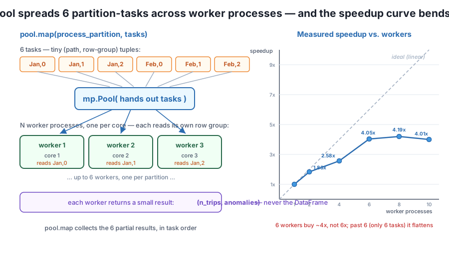
Pool hands six tiny (path, row‑group) tasks to worker processes spread across cores; each worker reads its own row group and returns only a small (n_trips, anomalies) tuple, never the DataFrame. Right: the measured speedup on ~6 million trips climbs steeply at first (1.83× at 2 workers, 2.58× at 4) but bends far below the dashed ideal line and flattens near 4× from 6 workers on — six processes buy about four times the throughput, and past six workers there are no more tasks to hand out, so nothing improves.pool.map is the right default, but it has two behaviors worth understanding. It returns results in input order, and it does not return anything until every task is done — it collects the whole list first. For six partitions that is fine. But when you have thousands of tasks, or you want to react to results as they land, two siblings help.
imap returns a lazy iterator that yields results one at a time, still in input order, as they become available — so you can start processing early results while later ones are still computing, and you never hold the full result list in memory at once. imap_unordered drops the ordering guarantee and yields each result the moment its worker finishes, whichever task that is. For a progress readout, or when order does not matter and you want the fastest possible turnaround, imap_unordered is ideal:
import warnings; warnings.filterwarnings("ignore")
import multiprocessing as mp
import pyarrow.parquet as pq
from datetime import datetime

def process_partition(args):
    path, i = args
    cols = ["tpep_pickup_datetime", "tpep_dropoff_datetime", "trip_distance", "fare_amount"]
    t = pq.ParquetFile(path).read_row_group(i, columns=cols).to_pandas()
    n = 0
    anomalies = 0
    for p, d, dist in zip(t["tpep_pickup_datetime"].astype(str),
                          t["tpep_dropoff_datetime"].astype(str),
                          t["trip_distance"]):
        mins = (datetime.fromisoformat(d) - datetime.fromisoformat(p)).total_seconds() / 60.0
        mph = dist / (mins / 60.0) if mins > 0 else 0.0
        if mph > 80 or mins < 0:
            anomalies += 1
        n += 1
    return (n, anomalies)

if __name__ == "__main__":
    files = ["yellow_tripdata_2024-01.parquet", "yellow_tripdata_2024-02.parquet"]
    tasks = [(f, i) for f in files for i in range(pq.ParquetFile(f).metadata.num_row_groups)]
    grand_total = 0
    with mp.Pool(processes=6) as pool:
        for n, anomalies in pool.imap_unordered(process_partition, tasks, chunksize=1):
            grand_total += n
            print(f"a partition finished: {n:>9,} trips, {anomalies:>4} anomalies")
    print(f"grand total: {grand_total:,} trips")
a partition finished: 867,472 trips, 375 anomalies
a partition finished: 910,374 trips, 236 anomalies
a partition finished: 1,048,576 trips, 409 anomalies
a partition finished: 1,048,576 trips, 379 anomalies
a partition finished: 1,048,576 trips, 343 anomalies
a partition finished: 1,048,576 trips, 381 anomalies
grand total: 5,972,150 tripsNotice the order: the two smaller row groups (867,472 and 910,374 rows) reported first, because they had less work and their workers finished sooner — that is imap_unordered handing you results in completion order, not input order. Run it again and the order can shuffle, since it depends on exactly which worker wins the race; the grand total, of course, is always the same 5,972,150. If you needed the results tied back to their input partition, you would use imap (ordered) or include an id in the return value.
The chunksize argument controls how many tasks the pool hands a worker at a time. The default is 1, meaning each worker fetches one task, finishes it, then asks for the next. For a small number of heavy tasks — our six fat partitions — chunksize=1 is exactly right: you want each partition dispatched independently so the pool can balance them. But when you have many tiny tasks (say a hundred thousand one-row jobs), a chunksize of 1 means a hundred thousand round-trips of scheduling overhead, and bumping it to a few hundred lets each worker grab a batch and amortize that cost. The principle is the mirror image of the task-size rule: match chunksize to task granularity — big tasks want chunksize=1, swarms of tiny tasks want a larger chunk.
The sweep already answered this for CityFlow, but the reasoning generalizes. This machine reports its core count directly:
import os
if __name__ == "__main__":
    print("logical cores:", os.cpu_count())
logical cores: 10Ten logical cores, and yet the job peaked around six workers and gained nothing past eight. Two ceilings are at play, and the lower one wins. The first ceiling is physical: a worker process needs a core to run on. Spin up more workers than cores and they take turns time-slicing the same cores, adding context-switching cost without adding real parallelism — which is why ten workers came out slower than eight here. The second ceiling is the number of tasks: with only six partitions, the seventh through tenth workers have no task to claim and contribute only startup overhead. For this job the task ceiling (6) bites before the core ceiling (10), so six workers is the sweet spot.
The honest takeaway is that the best worker count is measured, not assumed. A common starting guess is “as many workers as cores,” but that can be wrong in both directions: too high when you have fewer tasks than cores (like here), and sometimes too low when tasks spend time waiting on I/O and a core can usefully juggle more than one. The sweep you ran is the real answer — for this workload, on this machine. When the workload or the box changes, re-run it.
Leave a core for everything else
On a shared or interactive machine, a common production choice is processes=os.cpu_count() - 1 rather than the full count — it leaves one core for the operating system, your progress logging, and the parent process that is gathering results, which keeps the whole box responsive and often improves wall-clock time by avoiding oversubscription. As always, if it matters, measure both.
__main__ GuardYou have seen if __name__ == "__main__": wrapped around every pool in this lesson. It is not a stylistic habit — under the default start method on macOS and Windows, it is mandatory, and leaving it off breaks the program spectacularly.
Here is why. When you create a Pool, Python starts the worker processes with the spawn start method, which launches a fresh Python interpreter for each worker and has it re-import your script module to get access to your functions (that is how the worker finds process_partition — it imports it by name). Re-importing runs every line at the top level of your file. If your pool-creating code sits at the top level, each spawned worker will re-run it — creating its own pool of workers, which each re-import and create their own pools, and so on. The result is an explosion of processes and a crash. The if __name__ == "__main__": guard is what stops it: when the parent runs your file directly, __name__ is "__main__" and the guarded block runs; when a worker re-imports the file, __name__ is the module’s name instead, so the guarded block is skipped and the worker just picks up the function definitions it came for.
The guard is required — and it is why we run these as scripts
Because every worker re-imports the module under spawn, two rules are absolute: worker functions must be defined at the top level (so they are importable and picklable — a function nested inside another function cannot be pickled), and all pool creation, timing, and printing must live inside if __name__ == "__main__": (so it runs only in the parent, never in a re-importing worker). This is also why multiprocessing code is written as a .py script and run from the terminal rather than typed into a notebook cell — a notebook has no importable __main__ module for the workers to re-import, so pools built interactively often fail or hang. Write pipeline.py, keep the top level to imports and defs, and run it with python pipeline.py.
Exercise 1 — Run the sweep and read the curve. Using the process_partition worker and the six-task list, time the job at 1 (serial), 2, 4, and 6 workers, and print a workers / seconds / speedup table where speedup is the serial time divided by each parallel time. Confirm the shape: a real speedup at 2 and 4 workers that is clearly less than 2× and 4×, climbing to roughly 4× at 6. Note in a comment that your exact seconds will differ from the lesson’s.
Hint
Build tasks = [(f, i) for f in files for i in range(pq.ParquetFile(f).metadata.num_row_groups)]. Time the serial baseline with a plain list comprehension over process_partition, wrapped in time.perf_counter() calls. For each worker count, open with mp.Pool(processes=n) as pool: and call pool.map(process_partition, tasks). Keep the whole timing loop inside if __name__ == "__main__":.
Exercise 2 — Report partials as they finish with imap_unordered. Rewrite the job to use pool.imap_unordered(process_partition, tasks) with six workers, and print each (n_trips, anomalies) partial the moment it arrives, accumulating a running grand total. Confirm the grand total is 5,972,150 trips regardless of the order the partials print in, and explain in a comment why the two smaller row groups tend to report first.
Hint
imap_unordered returns an iterator, so loop over it directly: for n, anomalies in pool.imap_unordered(process_partition, tasks):. Add n to a running total inside the loop and print after. The smaller partitions (about 867k and 910k rows) carry less per-trip work, so their workers finish sooner and their results surface first — that is completion order, not input order.
Exercise 3 — Find your machine’s sweet spot. Extend the sweep to include 8 and 10 workers (and, if your machine has more cores, beyond). Print the full table and identify the worker count with the best speedup. Then, in a comment, explain the two ceilings that stop it from scaling to your full core count: the number of tasks (only six partitions) and the number of physical cores.
Hint
Loop for n_workers in [1, 2, 4, 6, 8, 10]: (treat 1 as the serial baseline, or run it separately). Compare os.cpu_count() to the worker count where speedup stops improving. With only six tasks, workers seven and beyond have no partition to claim; and past your physical core count, workers time-slice and add overhead — whichever limit is lower is the one you hit first.
You turned Lesson 1’s one-off result into a tool you can drive and measure. multiprocessing.Pool(processes=N) gives you a team of N worker processes, and pool.map(worker, tasks) distributes the tasks across them and gathers the results in order — the two-line core of CPU parallelism. The judgment lives in the design: you made each task a tiny (path, row_group) tuple and let each worker read its own partition and return a small (n_trips, anomalies) result, so a million-row DataFrame never crosses a process boundary. Sweeping the worker count from 1 to 10 on ~6 million trips produced a genuinely sublinear curve — about 1.83x at 2 workers, 2.58x at 4, and 4.05x at 6, then flat through 8 and slightly worse at 10 — because the six unequal partitions cause load imbalance and, with only six tasks, extra workers have nothing to do. You met imap and imap_unordered for streaming results as they finish, saw why chunksize=1 fits a few heavy tasks while many tiny tasks want a larger chunk, learned to pick a worker count from the measured curve rather than a guess, and wrote the if __name__ == "__main__": guard that keeps a spawned pool from recursively re-launching itself.
mp.Pool(processes=N) + pool.map — a pool of N worker processes; map hands out tasks and collects results in input order. The workhorse of CPU-bound parallelism.(path, row_group)) and let the worker read its own data and return a small result; never pickle a big DataFrame across the process boundary.map vs imap vs imap_unordered — map returns everything in order after all tasks finish; imap yields lazily in order; imap_unordered yields each result the instant its worker finishes. chunksize batches tasks per worker — keep it 1 for a few heavy tasks, raise it for many tiny ones.__main__ guard is mandatory — under spawn, workers re-import the module, so worker functions must be top-level and all pool/timing/print code must sit inside if __name__ == "__main__":. This is why multiprocessing is written as a script.Parallelism is the first tool that lets CityFlow’s pipeline use the whole machine instead of one core while nine sit idle, and a Pool is how you reach for it in a dozen lines. But this lesson’s real lesson is the curve: adding workers buys progressively less, and past a point buys nothing, so the professional move is to measure the speedup for your actual workload and choose the worker count from evidence — the difference between “I threw ten processes at it” and “six workers gave the best wall-clock time, here is the table.” Just as important is the discipline the structure forces: tiny tasks, small results, top-level workers, and the __main__ guard. Get those right and the same six-partition pattern scales from a laptop to a many-core server; get them wrong and you pay to copy DataFrames between processes, or watch a script fork-bomb itself. You now have a working, measured pool — but pool.map returned a list of partials that you summed by hand. Giving that “split the work, then combine the pieces” pattern a name and a proper structure is the next step.
Look back at how each sweep ended: the workers each returned a small partial — a count, an anomaly tally — and the parent combined them with a plain sum(...). That two-phase shape, compute an independent partial for every partition in parallel, then merge the partials into the final answer, is not a one-off trick; it is a named, reusable pattern called MapReduce, and it is the backbone of nearly every distributed data system. In Lesson 3, The MapReduce Pattern, you will structure a real per-zone fare aggregation this way: a map step that runs process_partition across the six row groups to produce a small per-zone partial frame from each, and a reduce step that combines those partials with pd.concat(...).groupby(level=0).sum() into the final per-zone result. You will also prove the parallel answer is bit-for-bit identical to the serial one, and see the subtle reason a mean must be reduced as separate sums and counts rather than by averaging the averages. The pool you built here is the engine; MapReduce is the shape you pour the work into.
Keep DATATWEETS free. Help fund practical data, AI, and engineering lessons for learners worldwide.

