Title here
Summary here
In Lesson 2 you drove a multiprocessing Pool and watched six processes chew through the six NYC taxi partitions in roughly a quarter of the serial time. But that example counted anomalies — each worker returned a single number, and combining six numbers was a one-line sum(). Real pipelines rarely want a single number. CityFlow’s dashboard needs the average fare per pickup zone: 261 separate answers, one for each taxi zone in the city. The moment a parallel job produces a table of results instead of a scalar, you need a discipline for splitting the work and, just as importantly, for putting the pieces back together correctly.
That discipline is map-reduce, and you have already met half of it. In Module 4 you computed a running per-zone summary by streaming one chunk at a time: each chunk contributed a partial sum and a partial count, and you added those partials into a growing total. Map-reduce is that same idea with the chunks processed in parallel instead of one after another. The MAP step computes a small partial result for each partition independently — perfect for a Pool, because the partitions never look at each other. The REDUCE step combines those partials into the final answer. Get the shape right and the parallel result is provably identical to the serial one; get it wrong and you can be off by eighteen dollars a trip without any error being raised. This lesson builds it correctly and proves it.
By the end of this lesson, you will be able to:
map_partition worker that returns a small per-zone partial frame, not raw datapd.concat(...).groupby(level=0).sum() and derive the final meanYou will run every block as a script, because — as in Lesson 2 — multiprocessing under macOS spawn needs an importable, top-level worker and an if __name__ == "__main__": guard. Let’s split an aggregation.
Here is the whole pattern in one sentence: run a function on every partition to get a small partial result (map), then merge the partials into one final result (reduce). The reason this parallelizes so well is that the map step is embarrassingly parallel — each partition is processed with no knowledge of any other, so six processes can run six maps at literally the same time. The reduce step is small and serial, because by the time you reduce, each partition has already been boiled down from a million rows to a couple hundred.
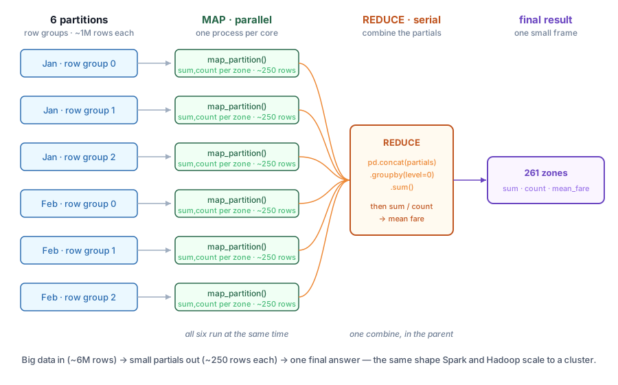
map_partition on each partition in parallel — one process per core — and every worker returns a small per-zone partial of roughly 250 rows, never the million-row partition itself. The single REDUCE step (orange) runs once in the parent process: it concatenates the six partials, groups by zone, sums the per-zone sum and count columns, and divides to get the mean fare. Roughly six million rows in, one 261-row answer out — the same shape Spark and Hadoop scale from your laptop's cores to a cluster.The key design decision is what the map step returns. A worker must never hand back its million-row partition — moving that much data out of a process is exactly the serialization cost Lesson 4 measures, and it would erase the parallel win. Instead each worker returns a small partial: the per-zone sum and count, which for the taxi data is about 250 rows regardless of how many million rows went in. Big data goes into the worker; a tiny summary comes out. That asymmetry is what makes the pattern fast and what makes the reduce step cheap.
The map worker reads its own row group — identified by a (path, row_group) tuple, so nothing large is pickled to it — and returns a per-zone partial. Instead of computing a mean directly, it returns the two combinable ingredients of a mean: the sum of fares and the count of trips per zone. (Why not the mean itself? That question has a costly answer we will get to.) Run the worker on a single partition first, so you can see the shape of what it produces:
import warnings; warnings.filterwarnings("ignore")
import pyarrow.parquet as pq

def map_partition(args):
    path, row_group = args
    df = pq.ParquetFile(path).read_row_group(
        row_group, columns=["PULocationID", "fare_amount"]).to_pandas()
    return df.groupby("PULocationID")["fare_amount"].agg(["sum", "count"])

if __name__ == "__main__":
    partial = map_partition(("yellow_tripdata_2024-01.parquet", 0))
    print("rows read from this partition :", partial["count"].sum())
    print("shape of the partial returned :", partial.shape)
    print(partial.head())
rows read from this partition : 1048576
shape of the partial returned : (247, 2)
sum count
PULocationID
1 12532.19 144
2 106.60 2
3 1663.00 33
4 14014.79 837
6 480.00 9The worker read 1,048,576 trips and returned a frame of just 247 rows — one per pickup zone that appeared in this partition, each carrying the total fare and the trip count for that zone. That is a reduction of more than four thousand to one before anything leaves the process. The index is PULocationID; the two columns are the partial sum and count. This is precisely the small, pickle-cheap result the map step should produce.
Return summaries, not rows
The single most important habit in map-reduce is that a worker returns a reduced result, not raw data. map_partition reads a million rows but returns about 250 — the groupby collapses the partition inside the worker, so only the summary crosses the process boundary. If you instead returned the filtered million-row frame, multiprocessing would serialize it, ship it to the parent, and deserialize it, and that transfer would usually cost more than the computation you parallelized. Map heavy, return light.
Now map over all six partitions with a Pool, exactly as in Lesson 2, and collect the six partial frames. The reduce step then stacks them and re-groups: pd.concat(partials) puts all six partials in one frame (with PULocationID values repeating across the six), and .groupby(level=0).sum() adds up the per-zone sum and count across partitions. One final division turns those combined totals into the mean fare per zone.
import warnings; warnings.filterwarnings("ignore")
import multiprocessing as mp
import pyarrow.parquet as pq
import pandas as pd

FILES = ["yellow_tripdata_2024-01.parquet", "yellow_tripdata_2024-02.parquet"]

def map_partition(args):
    path, row_group = args
    df = pq.ParquetFile(path).read_row_group(
        row_group, columns=["PULocationID", "fare_amount"]).to_pandas()
    return df.groupby("PULocationID")["fare_amount"].agg(["sum", "count"])

if __name__ == "__main__":
    tasks = [(f, i) for f in FILES
             for i in range(pq.ParquetFile(f).metadata.num_row_groups)]

    with mp.Pool(processes=6) as pool:          # MAP: 6 partitions, in parallel
        partials = pool.map(map_partition, tasks)

    combined = pd.concat(partials).groupby(level=0).sum()   # REDUCE: combine
    combined["mean_fare"] = combined["sum"] / combined["count"]

    print("partitions mapped :", len(partials))
    print("zones after reduce:", len(combined))
    print("total trips       :", int(combined["count"].sum()))
    print("\nBusiest pickup zones (by trips):")
    print(combined.sort_values("count", ascending=False)
                  .head(5)[["count", "mean_fare"]].round(2))
partitions mapped : 6
zones after reduce: 261
total trips : 5972150
Busiest pickup zones (by trips):
count mean_fare
PULocationID
161 290557 15.35
237 283508 12.31
132 272040 59.45
236 270465 12.84
162 212655 14.92Six partials went in; one 261-row table came out, covering 5,972,150 trips across both months. The busiest pickup zone is 161 — Midtown Center — with 290,557 trips at an average fare of $15.35, followed by Upper East Side South (237) and JFK Airport (132). JFK stands out immediately: a $59.45 mean fare, roughly four times its neighbors, because airport trips are long. The map step did the million-row work six ways in parallel; the reduce step did nothing but add up six small frames and divide. That division of labor — heavy and parallel, then light and serial — is the whole pattern.
Here is the crux of the entire lesson. Spreading work across processes reorders it: partition three might finish before partition one, and the reduce combines them in whatever order they arrive. For the result to be trustworthy, that reordering must not change the answer. So don’t take it on faith — compute the same aggregate a completely different way, serially, with no processes at all, and compare. The serial version reads every row into one frame and does a single groupby:
import warnings; warnings.filterwarnings("ignore")
import multiprocessing as mp
import pyarrow.parquet as pq
import pandas as pd

FILES = ["yellow_tripdata_2024-01.parquet", "yellow_tripdata_2024-02.parquet"]

def map_partition(args):
    path, row_group = args
    df = pq.ParquetFile(path).read_row_group(
        row_group, columns=["PULocationID", "fare_amount"]).to_pandas()
    return df.groupby("PULocationID")["fare_amount"].agg(["sum", "count"])

if __name__ == "__main__":
    tasks = [(f, i) for f in FILES
             for i in range(pq.ParquetFile(f).metadata.num_row_groups)]

    # PARALLEL map-reduce
    with mp.Pool(processes=6) as pool:
        partials = pool.map(map_partition, tasks)
    parallel = pd.concat(partials).groupby(level=0).sum()
    parallel["mean_fare"] = parallel["sum"] / parallel["count"]

    # SERIAL: one grouped pass over every row, no processes at all
    frames = [pq.ParquetFile(f).read_row_group(i, columns=["PULocationID", "fare_amount"]).to_pandas()
              for f in FILES for i in range(pq.ParquetFile(f).metadata.num_row_groups)]
    everything = pd.concat(frames, ignore_index=True)
    serial = everything.groupby("PULocationID")["fare_amount"].agg(["sum", "count"])
    serial["mean_fare"] = serial["sum"] / serial["count"]

    parallel = parallel.sort_index()
    serial = serial.sort_index()
    print("same set of zones      :", parallel.index.equals(serial.index))
    print("trip counts identical  :", parallel["count"].equals(serial["count"]))
    print("largest fare-sum gap    : {:.2e}".format((parallel["sum"] - serial["sum"]).abs().max()))
    print("largest mean-fare gap   : {:.2e}".format((parallel["mean_fare"] - serial["mean_fare"]).abs().max()))
same set of zones : True
trip counts identical : True
largest fare-sum gap : 4.66e-10
largest mean-fare gap : 7.11e-15This is the result the whole pattern rests on. The parallel map-reduce and the serial single-pass produce the same 261 zones, and the trip counts are bit-for-bit identical — counts are integers, and integer addition is exactly associative, so reordering it across processes changes nothing at all. The fare sums differ by at most 4.66e-10 — less than a billionth of a dollar across nearly six million trips. That residue is not a bug in the parallelism; it is floating-point addition, which is associative only to about fifteen digits, so summing the values in a different order nudges the last bit. The mean fares agree to 7.11e-15, essentially machine precision. For every practical purpose the parallel answer is the serial answer — and now you have proven it rather than assumed it.
Make the correctness check part of the pipeline
This serial-versus-parallel comparison is not just a one-time demo — it is a test worth keeping. Run it on a small partition (or a single month) in your test suite so that any future change to map_partition or the reduce logic must still reproduce the serial answer. Integer keys and counts should match exactly (.equals); floating-point sums should match to a tolerance like 1e-6, never with ==. A parallel aggregation you cannot reproduce serially is one you cannot trust.
The parallel answer matched the serial one because of a mathematical property, not luck. A reduction can be split across partitions and recombined in any order only if the combine operation is associative and commutative — that is, only if regrouping the terms and reordering them leaves the result unchanged. Formally, an operation is safe to parallelize when both hold for all partial results:
Sum, count, min, and max all satisfy this, so they reduce cleanly: the total is the sum of partial sums, the overall count is the sum of partial counts, the global maximum is the max of partial maxima. That is why map_partition returned sum and count and why the reduce was a plain .groupby(level=0).sum(). Mean is not directly combinable — you cannot average six partial averages and get the true average unless every partition has exactly the same number of rows. The fix is the one you used: reduce the ingredients of the mean (sum and count, which are each associative) and divide only at the very end. Watch what happens if you skip that discipline and naively average the six per-partition means:
import warnings; warnings.filterwarnings("ignore")
import multiprocessing as mp
import pyarrow.parquet as pq
import pandas as pd

FILES = ["yellow_tripdata_2024-01.parquet", "yellow_tripdata_2024-02.parquet"]

def mean_only(args):
    path, row_group = args
    df = pq.ParquetFile(path).read_row_group(
        row_group, columns=["PULocationID", "fare_amount"]).to_pandas()
    return df.groupby("PULocationID")["fare_amount"].mean()      # a mean per partition

def map_partition(args):
    path, row_group = args
    df = pq.ParquetFile(path).read_row_group(
        row_group, columns=["PULocationID", "fare_amount"]).to_pandas()
    return df.groupby("PULocationID")["fare_amount"].agg(["sum", "count"])

if __name__ == "__main__":
    tasks = [(f, i) for f in FILES
             for i in range(pq.ParquetFile(f).metadata.num_row_groups)]

    with mp.Pool(processes=6) as pool:
        mean_parts = pool.map(mean_only, tasks)
        sumcount_parts = pool.map(map_partition, tasks)

    # WRONG: average the six partial means (a mean of means)
    wrong = pd.concat(mean_parts).groupby(level=0).mean()

    # RIGHT: reduce sum and count, then divide once
    combined = pd.concat(sumcount_parts).groupby(level=0).sum()
    right = combined["sum"] / combined["count"]

    zone = 132   # JFK Airport
    print("mean of partial means (WRONG):", round(float(wrong.loc[zone]), 4))
    print("sum-then-count       (RIGHT):", round(float(right.loc[zone]), 4))
    print("largest per-zone error from mean-of-means:", round(float((wrong - right).abs().max()), 4))
mean of partial means (WRONG): 59.4085
sum-then-count (RIGHT): 59.4477
largest per-zone error from mean-of-means: 18.5403Averaging the six partial means gives JFK a mean fare of $59.41 where the true figure is $59.45 — and for some zone the mean-of-means is off by $18.54 a trip. No error is raised; the number is simply wrong, because the six partitions hold different numbers of trips for each zone and an unweighted average of their means silently ignores those weights. This is the same warning Module 4 raised about the median, which is worse still: a median cannot be reconstructed from partial medians at all, because it depends on the full ordering of every value, so there is no small partial that reduces cleanly. When you design a parallel aggregation, the first question is always: is my combine step associative and commutative? If not, decompose it into pieces that are.
What you built is not a toy version of a big idea — it is the idea. Hadoop MapReduce and Apache Spark (a later course) run this exact pattern: a map phase that computes partial results on partitions spread across many machines, a shuffle that groups partials by key, and a reduce phase that combines them. The only difference is scale. Your partitions are six parquet row groups on one laptop; a cluster’s partitions are thousands of blocks across hundreds of nodes. Because the shape is identical — independent map, then associative reduce — the same aggregation that runs on your ten cores runs, unchanged in structure, on a thousand-core cluster. Learning to think in map and reduce here is learning to think in the terms every distributed data system uses.
Why frameworks insist on this shape
Spark and Hadoop can only distribute your work because they require the reduce to be associative and commutative — that constraint is what lets them run partitions in any order, on any machine, and retry a failed one without redoing the rest. When a distributed framework asks you to express an aggregation as a reduce or a combine function, it is asking exactly the question this lesson asked: what small partial does each partition emit, and how do two partials merge? Answer that correctly on your laptop and the same code scales out.
Exercise 1 — Reduce a different pair of statistics. Write a map_partition worker that returns, per PULocationID, the total trip_distance and the trip count (use .agg(["sum", "count"]) on trip_distance). Map it over the six partitions with a Pool, reduce with pd.concat(...).groupby(level=0).sum(), derive the mean distance per zone, and print the five zones with the longest average trips (require at least 1,000 trips so a tiny zone doesn’t dominate).
Hint
The structure is identical to the fare example — only the column changes. Read columns=["PULocationID", "trip_distance"] in the worker, and after the reduce compute combined["sum"] / combined["count"]. Filter with combined[combined["count"] >= 1000] before sorting by mean distance descending.
Exercise 2 — Prove your reduction matches serial. Take your distance aggregation from Exercise 1 and prove it correct: compute the same per-zone mean distance serially by reading every partition into one frame and doing a single groupby, then compare. Print whether the zone sets match, whether the trip counts are identical, and the largest absolute gap in mean distance between the parallel and serial results.
Hint
Reuse the pattern from the correctness section: build parallel from the Pool and serial from one pd.concat(frames, ignore_index=True) followed by groupby. Sort both by index, then check parallel.index.equals(serial.index), parallel["count"].equals(serial["count"]), and (parallel["mean"] - serial["mean"]).abs().max(). Expect the counts to match exactly and the mean gap to be around 1e-12 or smaller.
Exercise 3 — Find a reduction that does not combine. For each of these four candidate statistics, decide whether it can be computed as an associative-and-commutative reduce over partitions, and in one sentence say why: (a) the maximum fare_amount per zone, (b) the number of distinct payment_type values per zone, (c) the total tip_amount per zone, (d) the median trip_distance per zone. Then implement the two that combine cleanly and verify them against serial; explain what small partial each of the other two would need (and why one of them still cannot be done exactly).
Hint
Max and sum are associative and commutative — implement (a) with .agg("max") reduced by .groupby(level=0).max(), and (c) with sum. Distinct-count (b) is not additive, but each partition can emit the set of payment types it saw and the reduce can union the sets, then count — combinable if the partials carry sets, not counts. Median (d) is the one that cannot be done exactly from small partials, for the same reason Module 4 flagged: it needs the full ordering of every value.
You learned to structure a parallel aggregation as map-reduce: a MAP step that computes a small per-partition partial independently (embarrassingly parallel, one process per core) and a REDUCE step that combines the partials into the final answer (small and serial). Your map_partition worker read a million-row row group and returned only a ~250-row per-zone frame of sum and count — mapping heavy and returning light, so nothing large crossed the process boundary. The reduce was pd.concat(partials).groupby(level=0).sum() followed by one division for the mean fare, producing a 261-zone answer over 5,972,150 trips with Midtown Center the busiest pickup and JFK the priciest. Most importantly, you proved the pattern correct: the parallel result matched a serial single-pass with counts bit-for-bit identical and fare sums agreeing to within 5e-10. And you saw why the shape matters — reducing mean directly gives errors of over eighteen dollars a trip, because mean is not associative; you must reduce its associative ingredients (sum and count) and divide last.
sum/count frame), never the raw rows; this is the parallel, heavy step.pd.concat(...).groupby(level=0).sum(); because partials are tiny, the reduce is cheap and runs serially in the parent..equals and floating-point sums to a tolerance, never with ==.Map-reduce is the mental model that lets a data engineer reason about parallel and distributed aggregation without fear. Once you can look at an aggregation and immediately ask “what small partial does each partition emit, and is combining them associative?”, you can parallelize it correctly on the first try — and you can spot the traps, like averaging averages, that produce plausible-looking wrong numbers with no error message. For CityFlow, that discipline turns a per-zone fare summary from a single-core job that touches six million rows serially into six parallel maps and one tiny reduce, with a proof attached that the fast answer equals the slow one. And because the shape is identical to what Spark and Hadoop require, the thinking you practiced on ten cores is the same thinking you will use the day CityFlow’s data outgrows one machine.
You now have the correct shape for parallel aggregation, but there is a cost hiding in it that this lesson deliberately kept small: the price of moving data between processes. Every partial that crosses the boundary from a worker back to the parent must be serialized (pickled), shipped, and deserialized — and every task argument you send in is serialized too. So far you sent only a tiny (path, row_group) tuple in and got a ~250-row frame back, which is why the overhead stayed negligible and the parallelism paid off. In Lesson 4, Parallel Chunk Processing, you will combine chunking with parallelism directly and measure that serialization cost: what it actually takes to move a chunk of data to a worker versus letting the worker read its own chunk, and how that single decision determines whether adding processes speeds your pipeline up or quietly slows it down. It is the practical hinge on which real-world parallel data pipelines turn.
Keep DATATWEETS free. Help fund practical data, AI, and engineering lessons for learners worldwide.

