Lesson 4 - Parallel Chunk Processing

Welcome to Parallel Chunk Processing#

Two of CityFlow’s hardest-won techniques are about to meet. In Module 4 you learned to process the taxi data one partition at a time — reading a single parquet row group into memory, summarizing it, discarding it, and moving to the next. That kept memory flat no matter how large the file grew, but it ran on a single core: partitions were handled strictly one after another. Then Lessons 1 through 3 of this module showed that separate processes genuinely run in parallel, and drove a multiprocessing Pool over real taxi partitions to get nearly four times the throughput.

The obvious move is to combine them: hand each partition to a different worker process and summarize all six row groups at once. That works — but only if you avoid the one cost that quietly sinks most first attempts. Sending work to another process is not free. Every argument you pass and every value a worker returns is pickled (serialized to bytes), copied across the process boundary, and unpickled on the other side. A (path, index) tuple pickles to fifty bytes; a one-million-row DataFrame pickles to a hundred and forty megabytes. This lesson measures both, on the same six million trips, and shows that the difference decides whether parallelism pays off at all.

By the end of this lesson, you will be able to:

• Explain why passing arguments to worker processes incurs a pickle-serialize-copy-unpickle cost that shared-memory threads avoid
• Measure the two ways to feed a worker — passing a loaded DataFrame versus passing a (path, index) tuple — and show why the tuple keeps the full speedup
• Choose partition granularity by measuring load balance: too few big partitions idle your cores, too many tiny ones drown in per-task overhead
• Structure workers to return small aggregates rather than large frames, so the return trip does not re-incur the pickle cost
• Apply the mental model “move code to the data, not data to the code” that underlies distributed engines

Every partition here is a parquet row group — Jan 2024 and Feb 2024 have three each, six in all, about a million trips apiece. Let’s start by weighing what it costs to move one.

The Hidden Price Tag: Serialization#

When Module 4 processed a partition, the DataFrame lived in one process’s memory and stayed there. Multiprocessing breaks that. A worker is a separate Python process with its own memory space, so it cannot simply see a DataFrame the parent holds — the object has to be copied to it. Python does that copy by pickling: turning the object into a byte stream, sending those bytes through a pipe, and rebuilding the object on the other side. For a small argument this is instant. For a big DataFrame it is a real, measurable transfer.

Before running anything in parallel, weigh the two things you might hand a worker. Download the two months once from the official TLC source and save them next to your script:

# gate: skip
# The full months are public-domain NYC TLC trip records (~50 MB parquet each).
# Download once; the runnable blocks below read the local copies by name.
import urllib.request
for month in ["2024-01", "2024-02"]:
    url = f"https://d37ci6vzurychx.cloudfront.net/trip-data/yellow_tripdata_{month}.parquet"
    urllib.request.urlretrieve(url, f"yellow_tripdata_{month}.parquet")

Now measure what one partition costs to pickle as a DataFrame, versus the tiny tuple that would let a worker read it itself:

import warnings; warnings.filterwarnings("ignore")
import pickle
import pyarrow.parquet as pq

if __name__ == "__main__":
    partition = pq.ParquetFile("yellow_tripdata_2024-01.parquet").read_row_group(0).to_pandas()
    tuple_arg = ("yellow_tripdata_2024-01.parquet", 0)
    print(f"one partition: {len(partition):,} rows x {partition.shape[1]} columns")
    print(f"pickled as a DataFrame:      {len(pickle.dumps(partition)) / 1024 / 1024:.0f} MB")
    print(f"pickled as (path, index):    {len(pickle.dumps(tuple_arg))} bytes")

one partition: 1,048,576 rows x 19 columns
pickled as a DataFrame:      141 MB
pickled as (path, index):    50 bytes

There is the whole lesson in three lines. The same partition is either 141 megabytes of pickle or 50 bytes, depending on how you describe it to the worker. The DataFrame carries every value of every column; the tuple carries only where to find them. Feeding six workers the DataFrame way means shipping roughly 846 MB across process boundaries before any work starts. Feeding them the tuple way means shipping 300 bytes and letting each worker read its own partition from disk in parallel. Everything below measures how much that choice matters.

The Key Experiment: Two Ways to Feed a Worker#

Now measure it for real. The job is a genuine per-trip scan — CityFlow’s data-quality check that flags trips faster than 80 mph or with a negative duration, exactly the kind of heavy per-row Python work that parallelism helps (a plain vectorized aggregation would not, as you’ll see shortly). The worker function is the same computation in both cases. What differs is how it receives its partition.

The first worker, scan_partition_frame, is handed a whole DataFrame — the parent loads every partition and passes it. The second, scan_partition_path, is handed a (path, index) tuple and reads its own partition. Note the mandatory structure: both worker functions live at top level so they are importable under spawn, and all pool creation, timing, and printing sit inside if __name__ == "__main__":.

import warnings; warnings.filterwarnings("ignore")
import time, multiprocessing as mp
import pyarrow.parquet as pq
from datetime import datetime

SCAN_COLS = ["tpep_pickup_datetime", "tpep_dropoff_datetime", "trip_distance"]

def find_anomalies(frame):
    n = 0; anomalies = 0
    for pickup, dropoff, dist in zip(frame["tpep_pickup_datetime"].astype(str),
                                     frame["tpep_dropoff_datetime"].astype(str),
                                     frame["trip_distance"]):
        minutes = (datetime.fromisoformat(dropoff) - datetime.fromisoformat(pickup)).total_seconds() / 60.0
        mph = dist / (minutes / 60.0) if minutes > 0 else 0.0
        if mph > 80 or minutes < 0:
            anomalies += 1
        n += 1
    return (n, anomalies)

def scan_partition_frame(frame):          # BAD: worker is handed a whole DataFrame
    return find_anomalies(frame)

def scan_partition_path(task):            # GOOD: worker is handed (path, index), reads its own data
    path, i = task
    frame = pq.ParquetFile(path).read_row_group(i, columns=SCAN_COLS).to_pandas()
    return find_anomalies(frame)

if __name__ == "__main__":
    files = ["yellow_tripdata_2024-01.parquet", "yellow_tripdata_2024-02.parquet"]
    tasks = [(f, i) for f in files for i in range(pq.ParquetFile(f).metadata.num_row_groups)]

    start = time.perf_counter()
    serial = [scan_partition_path(t) for t in tasks]
    t_serial = time.perf_counter() - start
    trips = sum(r[0] for r in serial); anoms = sum(r[1] for r in serial)
    print(f"serial (one core)     {t_serial:6.2f}s   trips={trips:,}  anomalies={anoms:,}")

    start = time.perf_counter()
    partitions = [pq.ParquetFile(f).read_row_group(i).to_pandas() for (f, i) in tasks]
    read_time = time.perf_counter() - start
    start = time.perf_counter()
    with mp.Pool(processes=6) as pool:
        pool.map(scan_partition_frame, partitions)
    pool_time = time.perf_counter() - start
    t_frame = read_time + pool_time
    print(f"pass the DataFrame    {t_frame:6.2f}s   (parent read {read_time:.2f}s + pool {pool_time:.2f}s)")

    start = time.perf_counter()
    with mp.Pool(processes=6) as pool:
        pool.map(scan_partition_path, tasks)
    t_path = time.perf_counter() - start
    print(f"pass the path         {t_path:6.2f}s")

    print(f"\nspeedup: pass-the-DataFrame {t_serial/t_frame:.2f}x  |  pass-the-path {t_serial/t_path:.2f}x")
    print(f"pass-the-path is {t_frame/t_path:.2f}x faster than pass-the-DataFrame")

serial (one core)     12.75s   trips=5,972,150  anomalies=2,123
pass the DataFrame      4.12s   (parent read 0.26s + pool 3.86s)
pass the path           2.80s

speedup: pass-the-DataFrame 3.09x  |  pass-the-path 4.56x
pass-the-path is 1.47x faster than pass-the-DataFrame

Both approaches beat the 12.75-second serial baseline, but by very different margins. Passing the path reached 4.56x — essentially the full win six workers can give on this machine. Passing the DataFrame reached only 3.09x, and the whole gap is serialization: the parent had to pickle six partitions totalling 846 MB and push them through pipes to the workers, all while the workers waited for their data to arrive. That overhead threw away a third of the speedup — pass-the-path finished 1.47x faster doing the identical computation. The exact seconds shift a little run to run (this is a live measurement on a busy laptop), but the ordering is stable: the tuple always wins, because moving 50 bytes is always cheaper than moving 141.

Note a second, quieter advantage of the path approach. scan_partition_path reads only the three columns it needs (SCAN_COLS), while scan_partition_frame received all nineteen — the parent had already materialized the whole partition. Passing a path lets the worker be selective about what it even loads. Passing a frame forces you to serialize everything you happened to have in hand.

When the Work Is Cheap, Parallelism Loses Either Way#

The experiment above used deliberately heavy per-trip Python. That matters, because parallelism only pays when each partition carries enough work to dwarf the fixed costs of spawning a process and moving data. Swap the heavy scan for a cheap, C-level groupby — the kind of vectorized aggregation pandas already does in milliseconds — and the picture inverts:

import warnings; warnings.filterwarnings("ignore")
import time, pickle, multiprocessing as mp
import pyarrow.parquet as pq

AGG_COLS = ["PULocationID", "fare_amount", "tip_amount"]

def zone_totals(frame):
    return frame.groupby("PULocationID").agg(trips=("fare_amount", "size"),
                                             fare=("fare_amount", "sum"),
                                             tip=("tip_amount", "sum"))

def agg_from_frame(frame):
    return zone_totals(frame)

def agg_from_path(task):
    path, i = task
    return zone_totals(pq.ParquetFile(path).read_row_group(i, columns=AGG_COLS).to_pandas())

if __name__ == "__main__":
    files = ["yellow_tripdata_2024-01.parquet", "yellow_tripdata_2024-02.parquet"]
    tasks = [(f, i) for f in files for i in range(pq.ParquetFile(f).metadata.num_row_groups)]

    one = pq.ParquetFile(files[0]).read_row_group(0, columns=AGG_COLS).to_pandas()
    result = zone_totals(one)
    print(f"partition frame ({len(AGG_COLS)} cols): {len(pickle.dumps(one)) / 1024 / 1024:.0f} MB")
    print(f"per-zone result:        {len(result)} rows -> {len(pickle.dumps(result)) / 1024:.1f} KB")

    start = time.perf_counter()
    for t in tasks:
        agg_from_path(t)
    t_serial = time.perf_counter() - start
    print(f"\nserial                {t_serial:6.2f}s")

    frames = [pq.ParquetFile(f).read_row_group(i, columns=AGG_COLS).to_pandas() for (f, i) in tasks]
    start = time.perf_counter()
    with mp.Pool(processes=6) as pool:
        pool.map(agg_from_frame, frames)
    t_frame = time.perf_counter() - start
    print(f"pass the DataFrame    {t_frame:6.2f}s   ({t_serial/t_frame:.2f}x  -- slower than serial)")

    start = time.perf_counter()
    with mp.Pool(processes=6) as pool:
        pool.map(agg_from_path, tasks)
    t_path = time.perf_counter() - start
    print(f"pass the path         {t_path:6.2f}s   ({t_serial/t_path:.2f}x  -- still slower than serial)")

partition frame (3 cols): 20 MB
per-zone result:        247 rows -> 7.8 KB

serial                  0.14s
pass the DataFrame      0.57s   (0.25x  -- slower than serial)
pass the path           0.50s   (0.28x  -- still slower than serial)

Serial finished the whole six-partition aggregation in 0.14 seconds, because a groupby is optimized C code that never touches the Python interpreter per row. Both parallel versions were roughly four times slower — spawning six processes, importing modules in each, and moving data cost far more than the aggregation saved. Parallelism did not just fail to help; it actively hurt. This is the honest boundary of the technique: parallelize heavy per-partition Python, not work that is already fast. And even in this losing case, notice the path approach still edged out the DataFrame approach (0.50s vs 0.57s) — moving a 20 MB frame is still worse than moving a tuple, whichever side of the break-even line you land on.

Partition Granularity: The Load-Balance Sweet Spot#

Once you have committed to parallelism for genuinely heavy work, a second choice remains: how many partitions to split the job into. The natural unit is the parquet row group — six of them here. But you can go coarser (one task per file) or finer (slice each row group into pieces). Granularity controls load balance: how evenly the work spreads across your workers, and how much fixed overhead you pay per task.

Measure the spread. Below, a coarse split gives each worker a whole file; the natural split gives one row group per task; the finer splits cut each row group into equal row-range slices:

import warnings; warnings.filterwarnings("ignore")
import time, multiprocessing as mp
import pyarrow.parquet as pq
from datetime import datetime

SCAN_COLS = ["tpep_pickup_datetime", "tpep_dropoff_datetime", "trip_distance"]

def find_anomalies(frame):
    n = 0; anomalies = 0
    for pickup, dropoff, dist in zip(frame["tpep_pickup_datetime"].astype(str),
                                     frame["tpep_dropoff_datetime"].astype(str),
                                     frame["trip_distance"]):
        minutes = (datetime.fromisoformat(dropoff) - datetime.fromisoformat(pickup)).total_seconds() / 60.0
        mph = dist / (minutes / 60.0) if minutes > 0 else 0.0
        if mph > 80 or minutes < 0:
            anomalies += 1
        n += 1
    return (n, anomalies)

def scan_whole_file(path):                       # coarse: one task per file
    pf = pq.ParquetFile(path); trips = 0; anoms = 0
    for i in range(pf.metadata.num_row_groups):
        n, a = find_anomalies(pf.read_row_group(i, columns=SCAN_COLS).to_pandas())
        trips += n; anoms += a
    return (trips, anoms)

def scan_slice(task):                            # finer: a row-range slice of a row group
    path, i, start, stop = task
    frame = pq.ParquetFile(path).read_row_group(i, columns=SCAN_COLS).to_pandas().iloc[start:stop]
    return find_anomalies(frame)

def slice_tasks(files, slices_per_group):
    out = []
    for f in files:
        pf = pq.ParquetFile(f)
        for i in range(pf.metadata.num_row_groups):
            rows = pf.metadata.row_group(i).num_rows
            step = -(-rows // slices_per_group)   # ceiling division
            for s in range(0, rows, step):
                out.append((f, i, s, min(s + step, rows)))
    return out

if __name__ == "__main__":
    files = ["yellow_tripdata_2024-01.parquet", "yellow_tripdata_2024-02.parquet"]

    start = time.perf_counter()
    with mp.Pool(processes=6) as pool:
        pool.map(scan_whole_file, files)
    print(f"  2 tasks (whole files)      {time.perf_counter() - start:6.2f}s   (only 2 of 6 workers busy)")

    for spg, label in [(1, "(one row group each)"), (2, "(2 slices per group)"),
                       (4, "(4 slices per group)"), (16, "(16 slices per group)")]:
        tasks = slice_tasks(files, spg)
        start = time.perf_counter()
        with mp.Pool(processes=6) as pool:
            pool.map(scan_slice, tasks)
        print(f"{len(tasks):>3} tasks {label:<24} {time.perf_counter() - start:6.2f}s")

  2 tasks (whole files)        6.72s   (only 2 of 6 workers busy)
  6 tasks (one row group each)       2.84s
 12 tasks (2 slices per group)       2.90s
 24 tasks (4 slices per group)       3.33s
 96 tasks (16 slices per group)      3.75s

The shape of that column is the whole point. With only 2 tasks, just two of the six workers ever run; the other four sit idle the entire time, and the job takes 6.72 seconds — barely better than serial. Splitting into the 6 natural row groups puts every worker to work at once and drops it to 2.84 seconds, the sweet spot here. Going finer does not help: each slice re-reads its entire row group before discarding all but its slice, so 24 and 96 tasks pile on redundant reads and per-task dispatch overhead, climbing back to 3.33 and 3.75 seconds. There is a genuine minimum in the middle, and the only way to find it is to measure — the right granularity gives every core a full, roughly equal share of work without multiplying fixed costs.

The Return Trip Is Pickled Too#

Serialization is symmetric. You worked to pass workers a tiny 50-byte argument — but whatever each worker returns is pickled and shipped back to the parent the same way. Return a small aggregate and the trip home is free; return a big frame and you pay the 141 MB tax in reverse. Compare two workers doing identical read-and-aggregate work, differing only in what they hand back:

import warnings; warnings.filterwarnings("ignore")
import time, multiprocessing as mp
import pyarrow.parquet as pq

def combine_small(task):                 # same work, returns a small per-zone aggregate
    path, i = task
    frame = pq.ParquetFile(path).read_row_group(i).to_pandas()
    agg = frame.groupby("PULocationID").agg(trips=("fare_amount", "size"), fare=("fare_amount", "sum"))
    return agg

def combine_big(task):                   # same work, but ships the whole partition back
    path, i = task
    frame = pq.ParquetFile(path).read_row_group(i).to_pandas()
    agg = frame.groupby("PULocationID").agg(trips=("fare_amount", "size"), fare=("fare_amount", "sum"))
    return frame

if __name__ == "__main__":
    files = ["yellow_tripdata_2024-01.parquet", "yellow_tripdata_2024-02.parquet"]
    tasks = [(f, i) for f in files for i in range(pq.ParquetFile(f).metadata.num_row_groups)]

    start = time.perf_counter()
    with mp.Pool(processes=6) as pool:
        small = pool.map(combine_small, tasks)
    t_small = time.perf_counter() - start
    print(f"return a small aggregate   {t_small:6.2f}s   (workers send back {sum(len(s) for s in small):,} rows total)")

    start = time.perf_counter()
    with mp.Pool(processes=6) as pool:
        big = pool.map(combine_big, tasks)
    t_big = time.perf_counter() - start
    print(f"return the whole frame     {t_big:6.2f}s   (workers send back {sum(len(b) for b in big):,} rows total)")
    print(f"\nreturning big frames is {t_big / t_small:.1f}x slower on identical read + work")

return a small aggregate     1.34s   (workers send back 1,481 rows total)
return the whole frame       2.81s   (workers send back 5,972,150 rows total)

returning big frames is 2.1x slower on identical read + work

Both workers read the same partitions and computed the same groupby. The only difference is that combine_small returned 247-ish rows of per-zone totals — 1,481 rows across all six — while combine_big handed back all 5,972,150 trips. That return-trip pickle made it 2.1x slower for zero analytical gain. This is exactly the map-reduce shape from Lesson 3: each worker computes a small partial result, and the parent combines the partials. The reduce step wants small summaries, not raw data — a worker that returns a whole frame has quietly turned your map-reduce back into a data-shipping problem. Keep both ends of the trip small: pass a path in, return an aggregate out.

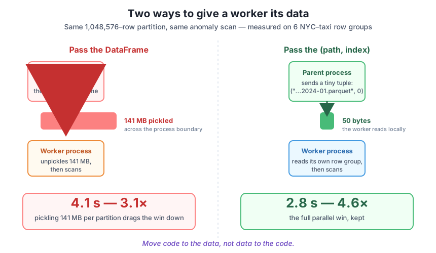
Practice Exercises#

Exercise 1 — Measure the payload difference yourself. Load a single row group of yellow_tripdata_2024-01.parquet into a DataFrame and, using pickle.dumps, print the size in megabytes of the frame versus the size in bytes of the (path, index) tuple that would let a worker read it. Then compute how many megabytes you would ship to feed all six partitions each way. Confirm the DataFrame route moves hundreds of times more data.

Exercise 2 — Prove pass-the-path wins on the heavy scan. Reuse find_anomalies, scan_partition_frame, and scan_partition_path from the key experiment. Time three runs over the six row groups: serial, a Pool fed loaded DataFrames, and a Pool fed (path, index) tuples. Print each time and the speedup versus serial, and confirm the tuple route is meaningfully faster than the DataFrame route. Remember to keep the worker functions at top level and everything else inside if __name__ == "__main__":.

Exercise 3 — Find your own granularity sweet spot. Using scan_whole_file, scan_slice, and slice_tasks from the granularity section, time the job at 2, 6, 12, 24, and 96 tasks on your machine and print each. Identify which task count is fastest for you, and explain in a comment why both the coarsest (idle cores) and finest (redundant reads plus per-task overhead) settings are slower than the middle.

Summary#

You combined Module 4’s chunking with Module 5’s parallelism and measured the cost that governs whether the combination pays off. A worker process shares no memory with the parent, so every argument and every return value is pickled, copied across the boundary, and unpickled. That made the way you feed a worker decisive: one taxi partition pickles to 141 MB as a DataFrame but 50 bytes as a (path, index) tuple. On six million trips of heavy per-trip work, passing the tuple hit the full 4.56x speedup while passing the DataFrame reached only 3.09x — a third of the win lost to shipping data the workers could have read themselves. When the per-partition work was cheap (a vectorized groupby), parallelism lost to serial outright, because spawn and pickle overhead dwarfed a sub-second computation. Granularity mattered too: two coarse tasks left four of six cores idle (6.72s), the six natural row groups balanced the load best (2.84s), and over-fine slices re-read their groups and climbed back up. And because the return trip is pickled as well, workers must return small aggregates — returning whole frames was 2.1x slower for no analytical gain.

Key Concepts#

• Serialization cost — arguments and return values crossing a process boundary are pickled, copied, and unpickled; the size of that payload, not the work, often decides whether parallelism helps.
• Pass a path, not a frame — hand workers a small (path, index) tuple and let each read its own partition; it keeps the full speedup and lets the worker load only the columns it needs.
• Parallelize heavy work only — per-partition Python (parsing, per-row logic) rewards parallelism; already-fast vectorized C aggregations lose to serial once spawn and pickle overhead are counted.
• Granularity is load balance — too few partitions idle cores, too many multiply per-task overhead and (if they cut across storage boundaries) force redundant reads; the sweet spot is found by measuring.
• Return small aggregates — the reduce step wants partial summaries, not raw data; returning big frames re-incurs the pickle cost on the way back and undoes the map-reduce.

Why This Matters#

The instinct that sinks a first parallel pipeline is to treat worker processes like function calls — load the data, hand it over, get results back — because that is exactly how single-process code works. In one process it is free; across processes it is a 141 MB copy each way. Internalizing “move code to the data, not data to the code” is what separates a parallel job that hits 4.5x from one that barely beats serial, or loses to it. For CityFlow it is the difference between a nightly summary that finishes in seconds and one that spends its time shuttling gigabytes between processes. It is also the exact principle behind the distributed engines you’ll meet later: Spark does not gather your data to one machine to compute — it ships the computation out to the machines where the data already lives, for precisely the reason you just measured. Passing a path is that idea in miniature.

Continue Building Your Skills#

You now have the full parallel-processing toolkit: processes over threads, a Pool, the map-reduce shape, and the serialization discipline that makes it all actually faster. Lesson 5, Measuring Speedup and Amdahl’s Law, turns the measuring you did here into a law. You saw six workers deliver 4.56x, not 6x — Lesson 5 explains exactly why, quantifying the ceiling with Amdahl’s law: the serial fraction of a job (reading, combining, the parent’s own work) caps how much any number of cores can help. Then the module’s guided project, Parallel Aggregation, Measured, puts everything together — you’ll parallelize Module 4’s per-zone, per-day summary job across the row groups, pass paths instead of frames, return small partials, and chart the speedup as you add workers until it visibly plateaus, watching Amdahl’s prediction play out on six million real trips.