Lesson 5 - Guided Project: Parallel Aggregation, Measured

Welcome to the Guided Project: Parallel Aggregation, Measured#

Across this module you learned what parallelism can and cannot do for a Python data job. You saw why the GIL keeps threads from speeding up CPU-bound work, why separate processes sidestep it, what it costs to hand data to a worker and get a result back, and how a Pool maps a function over many inputs. Each of those was a piece on its own. This project is where they become one measured pipeline.

You are a data engineer at CityFlow, and you already have the deliverable the dashboard team wanted: the per-zone, per-day taxi summary you built at the end of Module 4. It works, but it runs on a single core, one partition after another, while the other nine cores sit idle. Your job in this project is not to change what the summary computes — it is to make it faster by using every core, and then to prove, with a stopwatch, exactly how much faster. Not “parallel is faster” as an article of faith, but a real speedup number you measured yourself.

The honest twist is the one every engineer eventually meets: the speedup will be real but sublinear. Six worker processes will not make the job six times faster. This project builds the job, measures the curve, and then uses Amdahl’s law to explain the plateau you observe — so you leave knowing how to decide how many cores a job deserves, instead of guessing.

By the end of this project, you will be able to:

• Restructure a serial aggregation as a map-reduce over natural partitions
• Write a top-level worker that reads its own partition and returns a small partial result
• Reduce many partial summaries into one with concat and a grouped sum
• Measure speedup and efficiency across 1, 2, 4, 6, and 8 worker processes
• Estimate the parallelizable fraction with Amdahl’s law and predict the plateau

The job#

Everything runs on New York City’s public-domain Yellow Taxi trip records, published by the NYC Taxi & Limousine Commission (TLC) — the same two months you streamed in Module 4:

• January 2024, 2,964,624 rows: https://d37ci6vzurychx.cloudfront.net/trip-data/yellow_tripdata_2024-01.parquet
• February 2024, 3,007,526 rows: https://d37ci6vzurychx.cloudfront.net/trip-data/yellow_tripdata_2024-02.parquet

Each Parquet file is stored in 3 row groups of roughly a million rows, so the two months give you 6 natural partitions — and those 6 partitions are the unit of parallel work for the whole project. To attach human-readable names at the end you reuse the small zone lookup dimension (265 zones):

• Zone lookup: https://datatweets.com/datasets/nyc-taxi/taxi_zone_lookup.csv

In a real pipeline you download each month once and then read the local cached copy, so the runnable code below reads the bare local filenames — exactly as the pipeline does after caching:

# gate: skip
# The real public source: one Parquet file per month on the TLC CloudFront host.
BASE = "https://d37ci6vzurychx.cloudfront.net/trip-data/"
for month in ("2024-01", "2024-02"):
    print(BASE + f"yellow_tripdata_{month}.parquet")

There is one deliberate change from the Module 4 version of this summary, and it is the whole reason parallelism is worth it here. The old rollup let SQLite do the counting, which is fast C code — throwing more cores at fast C code wins you almost nothing once you pay for process startup. So this project makes the per-partition work genuinely CPU-bound in Python: for every one of the ~6 million trips it parses the two timestamp strings and computes the trip duration in minutes. Per-row datetime.fromisoformat over six million rows is real Python compute — seconds of it — and that is exactly the kind of work parallel processes speed up.

Stage 1: The MAP worker#

The map step is one function, defined at the top level of the script so every spawned worker can import it. It receives the smallest possible argument — a (path, row_group_index) tuple — and does everything else itself: it reads only its own row group (never the whole file), pulls just the four columns the summary needs, parses each trip’s two timestamps into a duration in minutes, derives the pickup date, and groups its ~1M rows down to a small partial summary of a few thousand rows.

That last point is the one that makes parallelism actually pay off. A worker never ships a million raw rows back to the parent — it ships back a grouped partial of a few thousand rows. Passing tiny arguments in and small results out is what keeps the pickling cost (which you measured earlier in this module) from eating the gains.

import warnings; warnings.filterwarnings("ignore")
import time, multiprocessing as mp
import pandas as pd
import pyarrow.parquet as pq
from datetime import datetime

FILES = ["yellow_tripdata_2024-01.parquet", "yellow_tripdata_2024-02.parquet"]
COLS = ["tpep_pickup_datetime", "tpep_dropoff_datetime", "PULocationID", "total_amount"]

def summarize_partition(args):
    """MAP: read one row group, parse durations (CPU-heavy), return a small partial."""
    path, i = args
    t = pq.ParquetFile(path).read_row_group(i, columns=COLS).to_pandas()
    durations, dates = [], []
    for p, d in zip(t["tpep_pickup_datetime"].astype(str),
                    t["tpep_dropoff_datetime"].astype(str)):
        pk = datetime.fromisoformat(p)                       # parse pickup timestamp
        durations.append((datetime.fromisoformat(d) - pk).total_seconds() / 60.0)
        dates.append(pk.date().isoformat())                 # derive pickup_date
    t = t.assign(duration_min=durations, pickup_date=dates)
    return t.groupby(["PULocationID", "pickup_date"]).agg(
        trips=("total_amount", "size"),
        total_minutes=("duration_min", "sum"),
        revenue=("total_amount", "sum"),
    )

Nothing runs yet — this block only defines the worker and a couple of tiny constants, which is exactly what belongs at top level. The heavy loop inside summarize_partition is the CPU-bound core: two fromisoformat calls and a subtraction for every trip. Multiply that by ~1M rows per partition and you have real seconds of Python work per partition, six partitions’ worth in total — the thing worth spreading across cores.

Stage 2: The REDUCE step#

Each worker returns a small frame indexed by (PULocationID, pickup_date). The reduce step stacks all six of them with pd.concat, then groups by that shared index and sums — so a zone-day that appears in three different partitions (because its trips landed in three different row groups) is correctly added up into one row. Only after the totals are combined does it derive the average duration, as total_minutes / trips; averaging has to happen after the sum, never before, or you would be averaging averages.

def reduce_partials(partials):
    """REDUCE: stack the partials, sum by (zone, day), then derive the average."""
    combined = pd.concat(partials).groupby(level=[0, 1]).sum()
    combined["avg_duration_min"] = combined["total_minutes"] / combined["trips"]
    return combined

This is the classic map-reduce shape: an expensive, embarrassingly parallel map over independent partitions, then a cheap reduce that runs once, in the parent, over a handful of small frames. The reduce is inherently serial — it needs every partial before it can combine them — and, as you will see when we reach Amdahl’s law, that unavoidable serial tail is part of why the speedup plateaus.

Stage 3: Run it serially and build the summary#

Before timing anything in parallel, run the whole map-reduce the plain way — a list comprehension over the six partitions in one process — to establish the serial baseline every speedup is measured against, and to produce the actual summary. This is also where you join the zone names and handle the same stray out-of-month dates Module 4 caught, so the result is a clean, dashboard-ready table.

if __name__ == "__main__":
    tasks = [(f, i) for f in FILES
             for i in range(pq.ParquetFile(f).metadata.num_row_groups)]
    print("partitions (row groups):", len(tasks))

    t0 = time.perf_counter()
    partials = [summarize_partition(a) for a in tasks]      # MAP, serially
    combined = reduce_partials(partials)                    # REDUCE
    serial = time.perf_counter() - t0
    print(f"serial map-reduce time: {serial:.2f} s")
    print("combined shape (raw):", combined.shape)

    # join zone names + filter stray out-of-month pickups (as Module 4 did)
    zones = pd.read_csv("taxi_zone_lookup.csv")
    summary = combined.reset_index()
    summary = summary[(summary["pickup_date"] >= "2024-01-01") &
                      (summary["pickup_date"] <= "2024-02-29")]
    named = summary.merge(zones, left_on="PULocationID",
                          right_on="LocationID", how="left")
    print("summary rows (clean):", named.shape[0])
    print("total trips aggregated:", int(combined["trips"].sum()))

    top = named.sort_values("trips", ascending=False).head(6)
    print(top[["PULocationID", "Borough", "Zone", "pickup_date",
               "trips", "revenue", "avg_duration_min"]].round(2).to_string(index=False))

partitions (row groups): 6
serial map-reduce time: 10.56 s
combined shape (raw): (13466, 4)
summary rows (clean): 13448
total trips aggregated: 5972150
 PULocationID   Borough           Zone pickup_date  trips   revenue  avg_duration_min
          161 Manhattan Midtown Center  2024-02-29   7498 186570.90             16.64
          161 Manhattan Midtown Center  2024-02-15   7083 169664.98             15.27
          161 Manhattan Midtown Center  2024-02-08   6970 177375.68             16.59
          161 Manhattan Midtown Center  2024-02-22   6828 169763.07             16.57
          161 Manhattan Midtown Center  2024-02-28   6766 161368.39             15.66
          161 Manhattan Midtown Center  2024-01-18   6763 165883.75             15.62

The map-reduce produces exactly what Module 4’s SQL rollup did — 5,972,150 trips in, a 13,466-row raw summary, 13,448 rows after dropping the 18 stray out-of-month zone-days — plus the new avg_duration_min field the CPU-heavy parse bought us. The busiest zone-days all belong to Midtown Center, with 6,700 to 7,500 pickups a day at an average trip of about 16 minutes. The result is correct; the only question left is how fast we can make it. That serial time — 10.56 seconds here — is the number to beat.

Stage 4: The measurement#

This is the heart of the project. The map step is embarrassingly parallel: the six partitions are independent, so a Pool of worker processes can run summarize_partition on several at once, and the reduce still runs once in the parent. You sweep the worker count — 1, 2, 4, 6, 8 — time each run end to end (map in parallel, then reduce), and turn each time into two numbers:

• speedup = serial time / parallel time (how many times faster than one core)
• efficiency = speedup / workers (what fraction of each added core you actually captured)

if __name__ == "__main__":
    results = {}
    for w in [1, 2, 4, 6, 8]:
        t0 = time.perf_counter()
        with mp.Pool(processes=w) as pool:
            parts = pool.map(summarize_partition, tasks)    # MAP across w processes
        _ = reduce_partials(parts)                          # REDUCE in the parent
        results[w] = time.perf_counter() - t0

    print(f"serial reference: {serial:.2f} s\n")
    print(f"{'workers':>7}  {'time (s)':>8}  {'speedup':>7}  {'efficiency':>10}")
    for w in [1, 2, 4, 6, 8]:
        el = results[w]; sp = serial / el
        print(f"{w:>7}  {el:>8.2f}  {sp:>6.2f}x  {sp/w:>9.2f}")

serial reference: 10.56 s

workers  time (s)  speedup  efficiency
      1     10.79    0.98x       0.98
      2      5.75    1.84x       0.92
      4      3.92    2.69x       0.67
      6      2.48    4.26x       0.71
      8      2.44    4.33x       0.54

Read that table slowly, because it is the whole lesson. One worker is a hair slower than serial (0.98x) — that is the cost of spawning a process and pickling results, with no parallelism to pay for it. Two workers land at 1.84x with 92% efficiency: nearly the full doubling, because the two processes stay busy and overhead is still small. But watch efficiency fall as you add cores: 0.67 at four, and although six workers reach the best speedup of 4.26x, that is only 71% efficiency — each core is now delivering less than three-quarters of a core’s worth of gain. And eight workers barely move the needle at all (4.33x), because there are only 6 partitions of work — the 7th and 8th workers have nothing to do but wait.

Stage 5: Amdahl’s law explains the plateau#

The table shows a plateau; Amdahl’s law tells you why, and lets you predict it. Any job splits into a part that can run in parallel (fraction $p$) and a part that is stubbornly serial (fraction $1 - p$) — here the serial part is the reading coordination, the process startup, the pickling of results, and the reduce that must wait for all six partials. If you run the parallel part on $N$ workers, the total time shrinks only on that fraction, and the best speedup you can get is:

You can estimate $p$ directly from a measured point. Rearranging the formula, $p = \dfrac{1 - 1/S}{1 - 1/N}$. The six-worker run is the fairest point to fit — with 6 partitions and 6 workers, each worker gets exactly one partition, so load is balanced and the measurement reflects the true parallel fraction rather than idle time. Plug in $S = 4.26$ at $N = 6$, then use that $p$ to predict the whole curve:

if __name__ == "__main__":
    def amdahl(p, n):
        return 1.0 / ((1 - p) + p / n)

    s6 = serial / results[6]                     # measured 6-worker speedup
    p = (1 - 1 / s6) / (1 - 1 / 6)               # solve Amdahl for p
    print(f"estimated parallelizable fraction p = {p:.3f}")
    print(f"serial fraction (1 - p)              = {1 - p:.3f}")
    print(f"theoretical ceiling S(inf) = 1/(1-p) = {1 / (1 - p):.1f}x\n")

    print(f"{'workers':>7}  {'Amdahl predicts':>15}  {'measured':>9}")
    for w in [1, 2, 4, 6, 8]:
        print(f"{w:>7}  {amdahl(p, w):>14.2f}x  {serial / results[w]:>8.2f}x")

estimated parallelizable fraction p = 0.918
serial fraction (1 - p)              = 0.082
theoretical ceiling S(inf) = 1/(1-p) = 12.2x

workers  Amdahl predicts   measured
      1            1.00x      0.98x
      2            1.85x      1.84x
      4            3.21x      2.69x
      6            4.26x      4.26x
      8            5.08x      4.33x

The fit is telling. About 92% of the work is parallelizable and roughly 8% is irreducibly serial — and that small serial slice is enough to cap the theoretical speedup at about 12x no matter how many cores you add. That is Amdahl’s blunt message: a job that is 8% serial can never go more than ~12 times faster, even on a thousand cores, because that 8% never shrinks.

Reality falls below even that ceiling for two concrete reasons visible in the gap between predicted and measured. At 4 workers, Amdahl’s optimistic 3.21x meets a measured 2.69x: 6 partitions across 4 workers means two workers handle 2 partitions each while two handle 1, so the busy pair gates the whole map phase — load imbalance across unequal partitions. At 8 workers, Amdahl predicts 5.08x but you measure 4.33x, because there are only 6 pieces of work — the extra two workers are pure overhead. Amdahl gives the optimistic envelope; granularity and imbalance pull you under it.

Stage 6: Wrap-up#

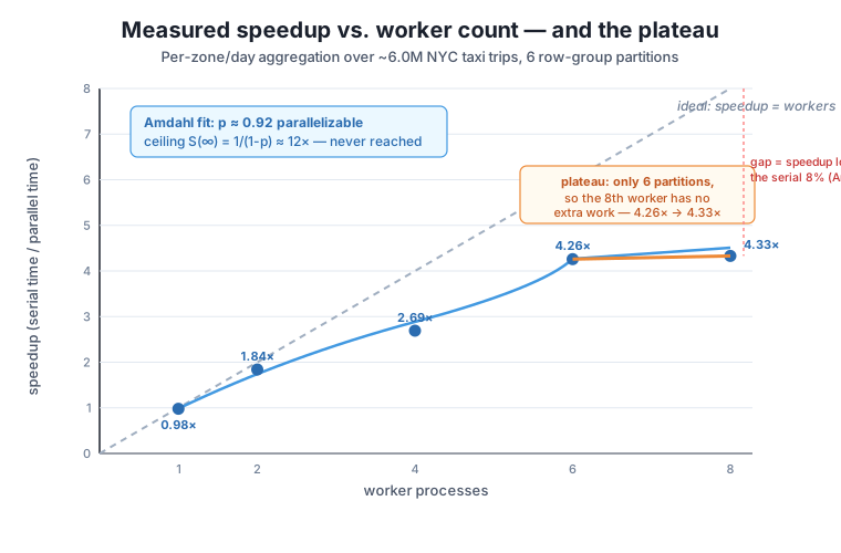
Step back and read the whole result as one measurement. You took the Module 4 summary — 5,972,150 trips in, a clean 13,448-row per-zone, per-day table out — added a genuinely CPU-bound duration field, and parallelized it as a map-reduce over 6 row-group partitions. Serially it ran in 10.56 s; the best parallel run, at 6 workers, finished in 2.48 s for a 4.26x speedup. Adding a 7th and 8th worker bought essentially nothing, because the work was already spread across all six partitions. Amdahl’s law, fit to the six-worker point, put the parallelizable fraction near 0.92 and predicted exactly the plateau you measured.

The takeaway is the one that separates a data engineer from someone who just knows the multiprocessing API: parallelism is a measured engineering decision, not a free multiplier. More cores do not mean proportionally more speed. The right number of workers is set by how much of your job is genuinely parallel, how many independent pieces of work you can split it into, and how much overhead each worker adds — and the only way to know it is to time the sweep, as you just did, and let the curve tell you where to stop.

Practice Exercises#

These extend the project you just built. Keep the top-level summarize_partition and reduce_partials exactly as they are, and reconnect to the same two local Parquet files.

Exercise 1. Add a third month and watch the partition count grow. Download March 2024 (yellow_tripdata_2024-03.parquet), add it to FILES, and rebuild tasks — you should now have 9 partitions instead of 6. Re-run the sweep out to 8 workers. Does the best speedup improve now that there are more independent pieces of work than before? What is the new efficiency at 8 workers compared to the 6-partition version?

Exercise 2. Add a live progress print with imap_unordered. Instead of pool.map (which blocks until every partition is done), use pool.imap_unordered(summarize_partition, tasks) and loop over the results as they arrive, collecting them into a list and printing f"partition {k} done" after each. Confirm the final reduce_partials on the collected list gives the identical 13,448-row summary. Why is imap_unordered safe to use here even though results come back out of order?

Exercise 3. Push to 10 workers and explain the result. Your machine has 10 logical cores; run the sweep with [6, 8, 10] workers on the original 6 partitions and compare. Does 10 workers beat 6? Write one sentence explaining the outcome in terms of both the partition count and Amdahl’s law.

Summary#

You parallelized Module 4’s per-zone, per-day taxi summary and measured the result honestly. The job — 5,972,150 trips over two months, 6 row-group partitions — was restructured as a map-reduce: a top-level summarize_partition worker reads one row group, parses each trip’s duration from its timestamp strings (the CPU-bound work that makes parallelism worthwhile), and returns a small grouped partial; reduce_partials then concatenates the partials and sums by (zone, day) to rebuild the exact 13,448-row clean summary. Timed across 1, 2, 4, 6, and 8 worker processes, the speedup rose from a near-linear 1.84x at 2 workers to a best of 4.26x at 6, then flattened — 8 workers gave 4.33x because there were only 6 partitions to share. Fitting Amdahl’s law to the 6-worker point estimated a parallelizable fraction of about 0.92, a serial fraction of about 0.08, and a theoretical ceiling near 12x that real overhead and load imbalance keep you well below.

Key Concepts#

• Map-reduce over partitions — an expensive, embarrassingly parallel map across independent pieces (here, 6 row groups) followed by one cheap serial reduce is the natural shape for parallelizing an aggregation.
• Small in, small out — workers receive a (path, index) tuple and return a few-thousand-row partial, never raw millions of rows, so pickling cost stays negligible and the parallel gain survives.
• Speedup and efficiency — speedup is serial time over parallel time; efficiency is speedup divided by workers. Watching efficiency fall as you add cores is how you spot diminishing returns.
• Amdahl’s law — $S(N) = 1 / ((1 - p) + p/N)$ caps speedup by the serial fraction $1 - p$; an 8% serial tail limits the job to about 12x no matter the core count.
• Granularity ceiling — you can never use more workers than you have partitions; six pieces of work cannot keep eight workers busy, which is a separate limit from Amdahl’s serial fraction.

Why This Matters#

Every scaling decision a data team makes eventually runs into this table. Someone asks for a job to be “twice as fast,” a well-meaning engineer throws all the cores at it, and the result is a 4x speedup on 8 cores that nobody can explain — or worse, a job that got slower because it was already fast C code and all the added cost went to process overhead. The skill you practiced here is the antidote: restructure the work into independent partitions, measure the speedup and efficiency across a range of worker counts, and use Amdahl’s law to understand the ceiling before you provision a bigger machine. That turns “add more cores” from a hopeful guess into an engineering decision backed by a curve — and it tells you the cheaper truth just as often, which is that a job is already as parallel as its structure allows and the next win has to come from somewhere else.

Continue Building Your Skills#

That completes Module 5: Parallel Processing. You now understand why the GIL blocks threaded CPU work, how processes sidestep it, what handing data to a worker really costs, how a Pool maps work across cores, and — as of this project — how to structure an aggregation as a map-reduce, measure its speedup and efficiency, and use Amdahl’s law to explain and predict where the gains run out.

There is a quieter lever underneath everything you have done, and it is where the course turns next. Notice that the reduce step leaned on grouping and joining — pairing each PULocationID with its zone name, adding up totals keyed by (zone, day). How fast those operations run depends entirely on the data structure holding the keys. Looking a value up in a Python list is a linear scan; looking it up in a dict or a set is effectively instant, no matter how many keys there are. Next comes Module 6: Data Structures for Data Work, where you make each individual access cheap: dicts and sets for O(1) lookups, deduplication, and fast joins, so the pipelines you have learned to stream and parallelize also spend their time wisely inside each step. Parallelism spreads the work across cores; the right data structure makes each piece of that work small in the first place.