Title here
Summary here
Module 6 ended on a genuine triumph. CityFlow’s zone lookup became a dict, and the cost of finding a zone stopped caring how many zones there were — \( O(1) \), 19.2x faster across all 2,964,624 January trips, paid for with a few kilobytes of deliberately empty hash slots. It was the module’s whole argument in one number, and it was true. So here is the uncomfortable question that opens Module 7: the dashboard’s next ticket asks for “every trip that started between 08:00 and 09:00.” You have a beautiful hash index. It is completely useless for this.
Not slow. Useless — as in, it has no better strategy than looking at every single key it holds. A hash table computes a slot from a key, and the whole point of a good hash is that it scrambles: it deliberately destroys any relationship between neighbouring keys so that they scatter into unrelated slots and collisions stay rare. That scattering is exactly what makes the exact-match lookup fast, and it is exactly why nothing about 08:00’s slot tells you where 08:01 lives. A range query needs the one property hashing throws away on purpose: order. Order is what the rest of this module buys, and order lives in trees — which is why every real database ships a B-tree index rather than only a hash. But a tree is a structure defined in terms of itself: a node holds children, and every child is a node holding children. Code that walks a structure like that wants to be shaped like the structure, and that shape is recursion. This lesson is the tool, before the structures that need it. You will measure the dict’s range-query failure (700x its exact-match cost), build CityFlow’s real 3-level zone hierarchy out of the TLC zone dimension and aggregate it recursively, and then get the honest news: recursion is not a performance trick, Python’s recursion limit is a real production constraint, and the rule that keeps you safe is one sentence long.
By the end of this lesson, you will be able to:
RecursionError in production: recurse on the structure’s depth, never on the data’s lengthYou’ll need pandas and Python’s standard library. Let’s find the dict’s limit.
The data is the public NYC TLC Trip Record Data — the same January 2024 yellow-taxi month the course has used throughout, plus the zone dimension that maps every LocationID to a zone, a service zone, and a borough. Fetch them once and keep them beside your script; every runnable block below reads the local copies by name:
# gate: skip
# CityFlow's month of trips plus the zone dimension, fetched once from public sources.
import urllib.request
urllib.request.urlretrieve(
    "https://d37ci6vzurychx.cloudfront.net/trip-data/yellow_tripdata_2024-01.parquet",
    "yellow_tripdata_2024-01.parquet",
)
urllib.request.urlretrieve(
    "https://datatweets.com/datasets/nyc-taxi/taxi_zone_lookup.csv",
    "taxi_zone_lookup.csv",
)
import warnings
warnings.filterwarnings("ignore")
import pandas as pd
import time
import sys
import math
from collections import Counter
zones = pd.read_csv("taxi_zone_lookup.csv").fillna("Unknown")
pickups = pd.read_parquet("yellow_tripdata_2024-01.parquet",
columns=["tpep_pickup_datetime", "PULocationID"])
print(f"zone dimension : {len(zones)} rows")
print(f"trips : {len(pickups):,}")
print(zones.head(3))zone dimension : 265 rows
trips : 2,964,624
LocationID Borough Zone service_zone
0 1 EWR Newark Airport EWR
1 2 Queens Jamaica Bay Boro Zone
2 3 Bronx Allerton/Pelham Gardens Boro ZoneNow build the index the dashboard actually wants — trips grouped by minute of day — and ask it two questions. One is the kind a hash was born for. The other is the kind it cannot do.
minute_of_day = (pickups["tpep_pickup_datetime"].dt.hour * 60
                 + pickups["tpep_pickup_datetime"].dt.minute)
by_minute = Counter(minute_of_day.tolist())
print("distinct minute-of-day keys:", len(by_minute))
print("dict key order is INSERTION order, not sorted:", list(by_minute)[:6])

def trips_between(index, lo, hi):
    return sum(n for minute, n in index.items() if lo <= minute < hi)

start = time.perf_counter()
for _ in range(20_000):
    by_minute[480]
exact_secs = time.perf_counter() - start

start = time.perf_counter()
for _ in range(20_000):
    trips_between(by_minute, 480, 540)
range_secs = time.perf_counter() - start

print(f"exact match  by_minute[480]        : {exact_secs / 20_000 * 1e6:8.3f} us  -> {by_minute[480]:,} trips")
print(f"range query  08:00 <= t < 09:00    : {range_secs / 20_000 * 1e6:8.3f} us  -> {trips_between(by_minute, 480, 540):,} trips")
print(f"the range query costs {range_secs / exact_secs:.0f}x the exact match")
distinct minute-of-day keys: 1440
dict key order is INSERTION order, not sorted: [57, 3, 17, 36, 46, 54]
exact match by_minute[480] : 0.071 us -> 1,602 trips
range query 08:00 <= t < 09:00 : 49.941 us -> 117,209 trips
the range query costs 700x the exact matchThere is Module 6’s triumph and Module 6’s ceiling, side by side. Asking “how many trips started exactly at 08:00?” costs 0.071 µs — one hash, one jump, 1,602 trips, and it would cost the same if the index held a million minutes. Asking “how many started between 08:00 and 09:00?” costs 49.941 µs, a 700x penalty, for an answer covering only 60 of the 1,440 keys.
Look at why in the second line of output. The dict’s keys come out in the order 57, 3, 17, 36, 46, 54 — insertion order, which is the order the first trip of each minute happened to appear in the file, and which is noise. Minute 480 and minute 481 are neighbours in every sense that matters to the dashboard and total strangers to the dict. So trips_between has no choice: it inspects all 1,440 keys and throws away 1,380 of them. That is \( O(n) \) in the size of the index — and note this is the good case, with only 1,440 keys. Index the month by second instead of minute and the same query gets 60 times worse while the exact match does not move at all.
This is not a flaw in Python’s dict. It is the definition of a hash table, and the cost of the thing that makes it fast. The fix is not a better hash; it is a different structure — one that keeps order, so that finding 08:00 also tells you where 08:01 is, and a range becomes a walk rather than a search. Those structures are trees, and Lessons 2 through 5 build them. But you cannot write a tree walk convincingly without recursion, so recursion is where we start.
Order is bought at build time, not query time
Keep this as the module’s through-line. Nothing gives you ordered access for free — the dict is fast because it refused to maintain order. Every structure in Module 7 pays for order somewhere, and it always pays up front: sorting the keys, keeping a tree balanced on insert, writing an index file next to your data. The bet is that you build once and query many times, which is the same bet Module 6’s zone_dict made and the same one that made it worth 19.2x. When the bet is wrong — one query, then throw the data away — a scan is genuinely the right answer, and knowing that is part of the job.
Before the mechanics, the honest framing — because recursion attracts more cargo-culting than any other idea in this course, and a beginner who meets it as a clever way to compute factorials learns the wrong lesson permanently.
In Python, recursion is almost always slower than the equivalent loop. There is no ambiguity about this and no tuning flag that changes it. Every recursive call builds a new stack frame: Python allocates it, binds the arguments, pushes it, and eventually pops and destroys it. A loop iteration does none of that — it jumps. Worse, as you will measure at the end of this lesson, Python enforces a hard ceiling on how many frames can be stacked at once, so a recursion that goes too deep does not merely run slowly; it raises an exception and dies. Languages built around recursion optimise the frames away. CPython does not, deliberately, and it is not going to.
So recursion is not on the menu for the same reason a dict was. Module 6’s dict earned its place with a measured 19.2x. Recursion earns its place a different way: when the data is nested, recursive code is dramatically clearer than the loop, at a cost near zero. That is the entire pitch, and it is worth taking seriously, because “clearer” is not a soft virtue in a pipeline that has to be debugged at 3am. There is exactly one case where recursion also buys real speed — divide-and-conquer, which turns \( O(n^2) \) into \( O(n \log n) \) — and we will measure that too, honestly, later in the lesson.
The test for “is this data nested?” is simple: can you say what one item is using the word for the thing itself? A zone tree is a node whose children are nodes. A JSON config is a value that may be a map of values. A filesystem is a directory of directories. When the definition curls back on itself, the code that reads it should curl back too — anything else means hand-writing the bookkeeping the language would do for you. When the data is a flat list of three million trips, it should not, and this lesson ends by measuring what happens to engineers who forget the difference.
Look again at the zone dimension. It has been sitting in the pipeline since Module 1 as a flat 265-row lookup table, but it has never actually been flat:
print(zones.groupby(["Borough", "service_zone"]).size())Borough service_zone
Bronx Boro Zone 43
Brooklyn Boro Zone 61
EWR EWR 1
Manhattan Boro Zone 14
Yellow Zone 55
Queens Airports 2
Boro Zone 67
Staten Island Boro Zone 20
Unknown Unknown 2
dtype: int64That is a genuine three-level hierarchy hiding in three CSV columns: 7 boroughs, each split into service zones (9 borough/service pairs in total), each holding the individual zones — 265 leaves. JFK Airport is not just zone 132; it is Queens → Airports → JFK Airport. That path is real geography and real taxi regulation (the “Yellow Zone” is where yellow cabs may pick up freely), and the dashboard’s drill-down wants exactly it.
A CSV cannot express a tree, so build one. Each node will be a dict: parents carry a children map, leaves carry a trips count.
zone_records = zones.to_dict("records")
trips_per_zone = Counter(pickups["PULocationID"].tolist())

def build_tree(records, leaf_key):
    root = {"name": "New York City", "children": {}}
    for r in records:
        borough = root["children"].setdefault(
            r["Borough"], {"name": r["Borough"], "children": {}})
        service = borough["children"].setdefault(
            r["service_zone"], {"name": r["service_zone"], "children": {}})
        service["children"][leaf_key(r)] = {
            "name": r["Zone"],
            "trips": int(trips_per_zone.get(r["LocationID"], 0)),
        }
    return root

tree = build_tree(zone_records, leaf_key=lambda r: r["Zone"])
print("root      :", tree["name"])
print("boroughs  :", list(tree["children"]))
print("Queens service zones:", list(tree["children"]["Queens"]["children"]))
print("one leaf  :", tree["children"]["Queens"]["children"]["Airports"]["children"]["JFK Airport"])
root : New York City
boroughs : ['EWR', 'Queens', 'Bronx', 'Manhattan', 'Staten Island', 'Brooklyn', 'Unknown']
Queens service zones: ['Boro Zone', 'Airports']
one leaf : {'name': 'JFK Airport', 'trips': 145240}The tree exists, and JFK’s 145,240 pickups — the busiest zone in the month, established back in Module 6 — are sitting at the end of a three-hop path. Notice the builder itself is a plain for loop with no recursion in it at all. Building a tree from flat rows is iterative; it is reading one that wants recursion, because reading is where you meet the self-similarity.
Every recursive function is two questions, and writing them down in order is the entire technique:
Our tree hands us both cases for free, because a node is exactly one of two things. A leaf has no children key — that is the base case, and its depth is obviously 1. A parent has children, and its depth is 1 plus the depth of its deepest child — the recursive case, in one line that reads almost exactly like the sentence.
def tree_depth(node):
    if "children" not in node:
        return 1
    return 1 + max(tree_depth(child) for child in node["children"].values())

def count_nodes(node):
    if "children" not in node:
        return 1
    return 1 + sum(count_nodes(child) for child in node["children"].values())

def count_leaves(node):
    if "children" not in node:
        return 1
    return sum(count_leaves(child) for child in node["children"].values())

print("tree depth  :", tree_depth(tree))
print("total nodes :", count_nodes(tree))
print("leaf zones  :", count_leaves(tree))
tree depth : 4
total nodes : 279
leaf zones : 262Three functions, three lines of logic each, and each one is the same skeleton: if leaf, answer directly; otherwise combine the children’s answers. Only the combining step differs — max for depth, 1 + sum for nodes, sum for leaves. That is the shape you are learning to recognise, and it is why the recursive version is worth the frames: the code is a transcription of the definition, with no stack, no queue, and no visited-set to get wrong.
Now use it for something CityFlow actually needs. The dashboard wants trips rolled up at every level — borough totals, service-zone totals — and that is the same skeleton again, with sum over a leaf’s trips:
def total_trips(node):
    if "children" not in node:
        return node["trips"]
    return sum(total_trips(child) for child in node["children"].values())

print(f"trips summed through the tree : {total_trips(tree):,}")
print(f"trips actually in the file    : {len(pickups):,}")
print(f"match                         : {total_trips(tree) == len(pickups)}")
print(f"missing                       : {len(pickups) - total_trips(tree):,}")
trips summed through the tree : 2,964,354
trips actually in the file : 2,964,624
match : False
missing : 270That is wrong, and I have left it wrong on purpose, because this is what the job is actually like. The tree says 2,964,354 trips. The file has 2,964,624. 270 trips fell out of the pipeline — and the reconciliation caught it only because we bothered to check the total against a number we already knew.
Look back at the previous output for the clue: leaf zones: 262. The dimension has 265 rows. Three leaves went missing, and with them 270 trips.
Nothing is wrong with total_trips. The recursion faithfully summed every leaf the tree contained; the tree simply contained three fewer leaves than it should. The suspect is build_tree, and specifically the leaf key:
path_counts = Counter((r["Borough"], r["service_zone"], r["Zone"]) for r in zone_records)
collisions = {path: n for path, n in path_counts.items() if n > 1}
print("zone paths that are not unique:")
for path, n in collisions.items():
    print(f"  {n}x  {path[0]} > {path[1]} > {path[2]}")
print()
for r in zone_records:
    if (r["Borough"], r["service_zone"], r["Zone"]) in collisions:
        print(f"  LocationID {r['LocationID']:3d}  {r['Zone']:45s}  {trips_per_zone.get(r['LocationID'], 0):>7,} trips")
zone paths that are not unique:
2x Queens > Boro Zone > Corona
3x Manhattan > Yellow Zone > Governor's Island/Ellis Island/Liberty Island
LocationID 56 Corona 270 trips
LocationID 57 Corona 10 trips
LocationID 103 Governor's Island/Ellis Island/Liberty Island 0 trips
LocationID 104 Governor's Island/Ellis Island/Liberty Island 0 trips
LocationID 105 Governor's Island/Ellis Island/Liberty Island 1 tripsThere it is, and it is entirely mundane. The zone name is not unique. Queens has two distinct zones both called “Corona” (LocationIDs 56 and 57), and Manhattan has three separate zones sharing the name “Governor’s Island/Ellis Island/Liberty Island” (103, 104, 105). Keying the leaf dict on r["Zone"] meant the second Corona overwrote the first — and since the loop processes ids in order, LocationID 56’s 270 trips were silently replaced by LocationID 57’s 10. The Governors Island trio collapsed the same way, but those zones have 0, 0, and 1 trips, so they cost only the leaf count, not the total. 270 + 0 = the exact deficit. The arithmetic closes.
This is worth more than the recursion lesson around it. setdefault and [key] = value do not warn you when a key repeats — a dict’s whole job is to hold one value per key, and it did that job perfectly. A natural-language name is not an identifier, no matter how much it looks like one, and a dimension table hands you the real identifier right there in column one. Key on the id:
tree = build_tree(zone_records, leaf_key=lambda r: r["LocationID"])
print("total nodes now :", count_nodes(tree))
print(f"trips summed through the tree : {total_trips(tree):,}")
print(f"trips actually in the file    : {len(pickups):,}")
print(f"match                         : {total_trips(tree) == len(pickups)}")
print()
print("pickups by borough, aggregated recursively:")
for name, node in sorted(tree["children"].items(), key=lambda kv: -total_trips(kv[1])):
    print(f"  {name:15s} {total_trips(node):9,}")
total nodes now : 282
trips summed through the tree : 2,964,624
trips actually in the file : 2,964,624
match : True
pickups by borough, aggregated recursively:
Manhattan 2,646,948
Queens 273,128
Brooklyn 25,258
Unknown 12,018
Bronx 6,905
EWR 295
Staten Island 72282 nodes, 265 leaves, and every one of the 2,964,624 trips accounted for. The borough totals now match Module 6’s dict-based enrichment exactly — Manhattan 2,646,948, Queens 273,128 — which is the reconciliation that proves the tree and the flat lookup agree. One lambda, 270 trips recovered, and a rule worth carrying: build the tree on ids, carry the names as labels.
Time to test the framing. Any recursion can be rewritten as a loop with an explicit stack — the loop just does by hand what Python’s call machinery was doing for you. Here is total_trips with the stack made visible, and both versions timed on the same real tree:
def total_trips_iterative(root):
    total = 0
    stack = [root]
    while stack:
        node = stack.pop()
        if "children" not in node:
            total += node["trips"]
        else:
            stack.extend(node["children"].values())
    return total

print("iterative total:", f"{total_trips_iterative(tree):,}")
print("same answer    :", total_trips_iterative(tree) == total_trips(tree))

REPEATS = 20_000
start = time.perf_counter()
for _ in range(REPEATS):
    total_trips(tree)
rec_secs = time.perf_counter() - start
start = time.perf_counter()
for _ in range(REPEATS):
    total_trips_iterative(tree)
itr_secs = time.perf_counter() - start
print(f"recursive walk : {rec_secs / REPEATS * 1e6:6.1f} us per full tree walk")
print(f"iterative walk : {itr_secs / REPEATS * 1e6:6.1f} us per full tree walk")
print(f"recursion costs {rec_secs / itr_secs:.2f}x the iterative version")
iterative total: 2,964,624
same answer : True
recursive walk : 26.5 us per full tree walk
iterative walk : 25.9 us per full tree walk
recursion costs 1.03x the iterative versionBoth walk all 282 nodes, both return 2,964,624, and the recursion costs 1.03x — about 3% — which is close enough to nothing that it would vanish between two runs on a busy laptop. So tell the truth about what this measurement shows, in both directions.
It does not show that recursion is fast. Look at the two functions. The iterative version had to invent a stack list, remember to pop, remember to extend, and get the leaf test right in a context where a mistake produces a wrong number rather than a crash. The recursive version says a node’s total is the sum of its children’s totals and stops. The recursion is the better code here by a wide margin and costs ~3%, and that is the trade you are actually being offered on nested data: near-zero cost for a large clarity win.
But notice why it is only 3%: the tree is 282 nodes and 4 levels deep. There are only 282 function calls in the whole walk, so there are only 282 frames to pay for, and the real work — the dict lookups, the sum, the generator — is identical in both. The frame overhead is small because the number of frames is small, and the number of frames is small because it is governed by the structure, not by the 2,964,624 trips the structure summarises. That is not a coincidence. It is the rule, and the next section shows what happens the moment you break it.
Here is the mistake, written in its most seductive form. Summing a list is a recursive-looking problem — the sum of a list is its first element plus the sum of the rest — and you can transcribe that sentence into Python without thinking twice:
tips = pd.read_parquet("yellow_tripdata_2024-01.parquet", columns=["tip_amount"])["tip_amount"].tolist()

def sum_tips_recursive(values, i=0):
    if i == len(values):
        return 0.0
    return values[i] + sum_tips_recursive(values, i + 1)

def sum_tips_iterative(values):
    total = 0.0
    for v in values:
        total += v
    return total

sample = tips[:900]
REPEATS = 2_000
start = time.perf_counter()
for _ in range(REPEATS):
    sum_tips_recursive(sample)
rec2 = time.perf_counter() - start
start = time.perf_counter()
for _ in range(REPEATS):
    sum_tips_iterative(sample)
itr2 = time.perf_counter() - start
print(f"same answer    : {abs(sum_tips_recursive(sample) - sum_tips_iterative(sample)) < 1e-9}")
print(f"recursive sum of 900 tips : {rec2 / REPEATS * 1e6:7.1f} us")
print(f"iterative sum of 900 tips : {itr2 / REPEATS * 1e6:7.1f} us")
print(f"recursion costs {rec2 / itr2:.2f}x the loop")
same answer : True
recursive sum of 900 tips : 85.9 us
iterative sum of 900 tips : 12.6 us
recursion costs 6.83x the loopIdentical answers, and now the frame overhead has nowhere to hide: 6.83x. This is the same language, the same machine, and the same 3% per-frame cost as the tree walk — but here the number of frames is 900 instead of 4, and the per-frame cost is all there is, since the “real work” is a single float addition. The tree walk hid the overhead behind useful work. This exposes it. That ratio alone should end the argument, but it is not even the serious problem.
print("sys.getrecursionlimit():", sys.getrecursionlimit())
survived = 0
died_at = None
for n in range(900, 1200):
    try:
        sum_tips_recursive(tips[:n])
        survived = n
    except RecursionError:
        died_at = n
        break
print(f"largest list this recursion could sum : {survived:,} trips")
print(f"RecursionError raised at              : {died_at:,} trips")
print(f"trips in the real month               : {len(tips):,}")
print(f"fraction of the month it could handle : {died_at / len(tips) * 100:.4f}%")

def sum_tips_tail(values, i=0, acc=0.0):
    if i == len(values):
        return acc
    return sum_tips_tail(values, i + 1, acc + values[i])

try:
    sum_tips_tail(tips[:5000])
    print("tail-recursive version survived 5,000")
except RecursionError:
    print("tail-recursive version ALSO dies: CPython does not optimize tail calls")

start = time.perf_counter()
total = sum_tips_iterative(tips)
print(f"the loop sums all {len(tips):,} tips in {time.perf_counter() - start:.2f} s: ${total:,.2f}")
sys.getrecursionlimit(): 1000
largest list this recursion could sum : 998 trips
RecursionError raised at : 999 trips
trips in the real month : 2,964,624
fraction of the month it could handle : 0.0337%
tail-recursive version ALSO dies: CPython does not optimize tail calls
the loop sums all 2,964,624 tips in 0.04 s: $9,889,600.31It dies at 999 rows. Not slowly — RecursionError, an exception, a failed job. Python’s sys.getrecursionlimit() is 1000 by default, and since each element costs one frame, this function’s entire universe is 998 trips: 0.0337% of one month. The loop it replaced sums all 2,964,624 in 0.04 s and reports January’s real tip take of \$9,889,600.31.
Two traps live in that output. The first is the temptation to reach for sys.setrecursionlimit(3_000_000), which is the worst available move: that limit is not a bureaucratic annoyance, it is a guard rail in front of the C stack, which is a fixed-size memory region Python does not manage. Raise the limit past what the stack can hold and you do not get an exception — you get a segmentation fault, a hard crash with no traceback, in production, at whatever data volume finally reaches it. Trading a clean error for a silent kill is not a fix.
The second is subtler and catches people who have read about functional languages. sum_tips_tail is written in tail-recursive form: the recursive call is the last thing it does, carrying the running total in an accumulator, so there is nothing left to compute after the call returns. In Scheme or Haskell a compiler would recognise that and reuse the frame, turning the recursion into a loop and making the depth free. CPython does not do this — and it is a deliberate, long-standing decision, not an oversight, because the maintainers value the complete stack traces those frames make possible. So the tail-recursive version dies exactly like the naive one. You cannot write your way around the limit; you can only stop needing it.
Which gives the rule, and it is the sentence to take away from this whole lesson:
Recurse on the depth of the structure, never on the length of the data. The zone tree is 4 deep no matter how many trips it summarises. A per-row recursion is as deep as the data, and the data always wins.
The depth question you must be able to answer
Before you ship any recursive function, answer this out loud: what is the maximum depth, and what determines it? If the answer names a structure — “the zone tree is 4 deep”, “our config nests at most 6 levels”, “log₂ of the input, so 22” — you are safe, and you can say why. If the answer is “however many rows we get” or “it depends on the file”, you have a production bug that will not appear in testing. Your test fixture has 50 rows; the recursion survives to 998; the pipeline meets 2,964,624 and raises RecursionError at 3am. The rewrite is nearly always a for loop, and it will also be faster.
So far recursion has bought clarity and cost 3%. There is one family of algorithms where it buys something a loop genuinely struggles to: divide-and-conquer. The shape is three steps — split the problem in half, solve both halves the same way, combine the results — and its recursive case calls itself twice rather than once, on inputs half the size.
Why that matters is worth stating before measuring. Halving is the most powerful move in this course. A per-row recursion on 2,964,624 rows needs 2,964,624 frames; a recursion that halves needs only as many levels as it takes to get from 2,964,624 down to 1 by repeated division — that is \( \log_2 n \), which is 22. The work at each of those 22 levels touches every element once, so the total is \( n \log_2 n \) rather than the \( n^2 \) you pay for comparing everything to everything.
Watch it on real tips. merge_sort is the canonical divide-and-conquer: split, sort each half recursively (a one-element list is already sorted — there is the base case), then merge the two sorted halves. Against it, insertion_sort, an honest \( O(n^2) \) loop. Double the input four times and read the columns:
def merge(left, right):
    out = []
    i = j = 0
    while i < len(left) and j < len(right):
        if left[i] <= right[j]:
            out.append(left[i]); i += 1
        else:
            out.append(right[j]); j += 1
    out.extend(left[i:])
    out.extend(right[j:])
    return out

def merge_sort(values):
    if len(values) <= 1:
        return values
    mid = len(values) // 2
    return merge(merge_sort(values[:mid]), merge_sort(values[mid:]))

def insertion_sort(values):
    out = list(values)
    for i in range(1, len(out)):
        key = out[i]
        j = i - 1
        while j >= 0 and out[j] > key:
            out[j + 1] = out[j]
            j -= 1
        out[j + 1] = key
    return out

print(f"{'n tips':>8} {'merge_sort':>12} {'insertion_sort':>16} {'ratio':>8} {'depth':>7}")
for n in (2_000, 4_000, 8_000, 16_000):
    sub = tips[:n]
    start = time.perf_counter(); a = merge_sort(sub); t_merge = time.perf_counter() - start
    start = time.perf_counter(); b = insertion_sort(sub); t_ins = time.perf_counter() - start
    assert a == b == sorted(sub)
    print(f"{n:8,} {t_merge * 1000:10.1f} ms {t_ins * 1000:13.1f} ms {t_ins / t_merge:7.1f}x {math.ceil(math.log2(n)):7d}")
n tips merge_sort insertion_sort ratio depth
2,000 3.1 ms 70.9 ms 22.6x 11
4,000 6.7 ms 284.4 ms 42.1x 12
8,000 14.4 ms 1157.9 ms 80.3x 13
16,000 30.4 ms 4893.6 ms 161.1x 14The assert confirms all three agree, so this is a like-for-like race. Now read the columns as sequences, which is the only way to read a complexity claim. merge_sort roughly doubles: 3.1, 6.7, 14.4, 30.4 — a touch more than doubling, which is the \( \log n \) factor creeping up one level at a time. insertion_sort quadruples: 70.9, 284.4, 1157.9, 4893.6. Double the input, pay four times — the same \( O(n^2) \) signature Module 6 found in a list-based in.
And so the ratio column is not a constant: 22.6x, 42.1x, 80.3x, 161.1x, roughly doubling each step. There is no single answer to “how much faster is merge sort” — only an answer at a size, growing without limit. This is recursion earning something no amount of micro-optimisation could: not a faster constant, a better exponent.
Look at the depth column, though, because it is the real point of putting this section after the RecursionError. Sorting 16,000 tips recursively needs a depth of 14. Sorting all 2,964,624 would need 22. Twenty-two frames, against the limit of 1000 — a 45x safety margin — to recursively sort a month of taxi trips. That is the difference between recursing on data length and recursing on a structure you created by halving. Divide-and-conquer is safe from the recursion limit for the same reason the zone tree is: its depth is logarithmic, and \( \log_2 \) of anything you will ever fit on a disk is a small number.
Treat this as the shape, not the destination. Real code calls sorted(), whose Timsort is a C implementation of the same divide-and-conquer idea and will beat both functions above. But the shape is about to become load-bearing: Lesson 2 applies halving to searching — bisect on a sorted array, the range query this lesson opened with, in \( O(\log n) \). Lesson 3 takes merge itself, the combine step you just wrote, and scales it to k-way merging with heapq.merge so CityFlow can sort files that never fit in memory. You have just written both of their engines in miniature.
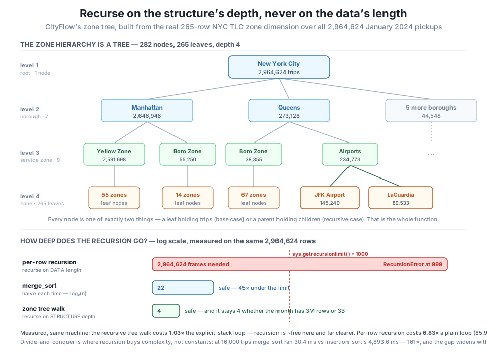
trips, or a parent holding children. Aggregating it recursively reconciles to all 2,964,624 January pickups (Manhattan 2,646,948, Queens 273,128), and JFK's 145,240 sit three hops down at Queens → Airports → JFK Airport. Bottom: depth is what decides whether a recursion survives. Recursing per row needs 2,964,624 frames and raises RecursionError at 999 — 0.0337% of the month — because sys.getrecursionlimit() is 1000 and CPython does not optimize tail calls. Recursing on a structure is safe: merge_sort halves, so it needs only 22 frames for the whole month, and the tree walk needs 4 forever. Measured: the recursive walk costs 1.03× the explicit-stack loop (clarity for ~3%), per-row recursion costs 6.83× a loop, and merge_sort beats insertion_sort 161× at 16,000 tips with the gap widening. Exact times vary by machine and run; the depths and ratios are the point.Put the three recursions of this lesson side by side and the decision procedure stops being a judgement call:
n_month = len(tips)
print(f"{'recursion':38s} {'depth needed':>14}  survives?")
print(f"{'per-row (recurse on DATA length)':38s} {n_month:>14,}  {'no':>9}")
print(f"{'merge_sort (halve each time)':38s} {math.ceil(math.log2(n_month)):>14,}  {'yes':>9}")
print(f"{'zone tree walk (STRUCTURE depth)':38s} {tree_depth(tree):>14,}  {'yes':>9}")
print(f"\nsys.getrecursionlimit() = {sys.getrecursionlimit():,}")
recursion depth needed survives?
per-row (recurse on DATA length) 2,964,624 no
merge_sort (halve each time) 22 yes
zone tree walk (STRUCTURE depth) 4 yes
sys.getrecursionlimit() = 1,000Three recursive functions over the same 2,964,624 trips. Two are safe by an enormous margin and one cannot run at all, and the discriminator is not style, cleverness, or how recursive the problem “feels” — it is a single number you can work out on paper before writing a line: what governs the depth? If it is the data, stop. If it is a structure — a hierarchy that is 4 deep, or a halving that gives you 22 — recurse, and enjoy the clearer code.
Exercise 1 — Recursive drill-down with paths. The dashboard needs more than borough totals: it needs a drill-down that prints the whole tree, indented, with each node’s trip total and its share of its parent. Write print_tree(node, depth=0, parent_total=None) that recurses through the corrected tree, indenting by depth, showing each node’s name, its total_trips, and its percentage of its parent (the root shows 100%). Prune the noise: skip any subtree with fewer than 1,000 trips and print a one-line (N zones below threshold) summary instead. Verify that Queens → Airports still shows 234,773 trips and that JFK’s 145,240 is 61.9% of it.
Hint
The base case and recursive case are the same two you have written four times now; only the action changes — print instead of sum. Pass depth down and use " " * depth for the indent, which is the standard way a recursion tracks where it is. Careful: calling total_trips(child) inside the print recursion re-walks each subtree, so the tree gets walked many times over — harmless at 282 nodes, and worth noticing as the same “build the index once” instinct from Module 6. If it bothers you, have the function return its own total on the way back up and print with it.
Exercise 2 — Find your own recursion limit, safely. The lesson found sum_tips_recursive dying at 999. Different functions die at different depths, because the limit counts frames, and a function with more locals or an extra helper call consumes them faster. Write max_safe_depth(fn) that takes a single-argument recursive function and, using a try / except RecursionError, finds the largest n it survives. Test it on sum_tips_recursive, on sum_tips_tail, and on a version that wraps each call in a tiny helper (return _add(values[i], sum_via_helper(values, i+1))). Report the three depths and explain the ordering. Do not call sys.setrecursionlimit().
Hint
Search upward in coarse steps and then refine, or binary-search between a known-good and known-bad n — this is itself the halving idea from the divide-and-conquer section, applied to a search. Always catch RecursionError specifically rather than a bare except, or you will swallow real bugs. Expect the helper version to die earliest: each level now costs two frames instead of one, so it should reach roughly half the depth. That is the lesson — the number 1000 is a budget in frames, and it is not always your function spending them.
Exercise 3 — Rewrite a data recursion as a loop, and prove it. Take sum_tips_recursive and write sum_tips_chunked(values, chunk=1000) that recurses on chunks rather than rows: if the list fits in one chunk, sum it with a plain loop (base case); otherwise split it in half and add the two halves’ results (recursive case). Confirm it produces \$9,889,600.31 on all 2,964,624 tips, measure its depth against sys.getrecursionlimit(), and time it against the plain loop. Then answer in a comment: it survives where the per-row version died — so is it a good idea?
Hint
Use math.ceil(math.log2(len(values) / chunk)) to predict the depth before you run it — it should land around 12, comfortably safe, because halving is halving whether the leaves are single rows or thousand-row chunks. On timing, be honest and expect to lose: you have added slicing and function calls around a loop that was already optimal, and the correct conclusion is that surviving is not the same as being worth it. This one is genuinely useful only when the chunks go somewhere else — different cores, as in Module 5, or different files, as in Lesson 3’s external sort.
Module 6’s hash index answers exactly one kind of question, and this lesson measured its ceiling: on the real January 2024 month, by_minute[480] costs 0.071 µs and the range query “08:00 to 09:00” costs 49.941 µs — 700x more for 117,209 trips — because a dict hands back its keys in insertion order (57, 3, 17, 36, 46, 54) and knows nothing about which keys are neighbours. Range queries need order, order lives in trees, and trees are recursive, so recursion came first. Every recursive function is a base case and a recursive case, and CityFlow’s zone dimension supplies both naturally: it is a real 3-level hierarchy — 7 boroughs, 9 service zones, 265 zones, 282 nodes at depth 4 — where a node is either a leaf with trips or a parent with children. Aggregating it recursively immediately caught a real bug: keying leaves on the zone name silently lost 270 trips, because Queens has two zones called “Corona” (LocationIDs 56 and 57) and Manhattan has three called “Governor’s Island/Ellis Island/Liberty Island” — a name is not an identifier. Keyed on LocationID the tree reconciles exactly to 2,964,624 and to Module 6’s borough totals. Then the honest measurements. Recursion is not a speed trick: the recursive tree walk costs 1.03x the explicit-stack loop, which is a ~3% price for much clearer code, and a per-row recursion costs 6.83x a plain loop (85.9 µs vs 12.6 µs over 900 tips) and raises RecursionError at 999 rows — 0.0337% of the month — since sys.getrecursionlimit() is 1000, CPython does not optimize tail calls, and raising the limit trades a clean exception for a segfault. Divide-and-conquer is where recursion earns real complexity: merge_sort roughly doubles (3.1 → 30.4 ms) while insertion_sort quadruples (70.9 → 4,893.6 ms), a ratio growing 22.6x → 161.1x — and its depth on the whole month would be just 22, versus the tree walk’s 4 and the per-row version’s impossible 2,964,624.
sys.getrecursionlimit() is 1000, so a per-row recursion over 2,964,624 trips dies at 999 (0.0337% of the month). Tail-recursive form does not help; CPython deliberately does not optimize tail calls, keeping full tracebacks instead. Raising the limit invites a C-stack segfault, which is strictly worse than an exception.merge_sort is 22 deep on the whole month because halving gives \( \log_2 n \). If you cannot name the structure that bounds your depth, the data is bounding it and you have a production bug.CityFlow’s pipeline has spent six modules getting fast at questions it can hash. This lesson is where the team admits there is a question it cannot, and it matters because “give me everything between X and Y” is not an exotic request — it is what a dashboard’s date picker is. The 700x gap between an exact match and a range query on the same index is the entire justification for Module 7’s existence, and recursion is the first tool on that road because the structures that preserve order are defined in terms of themselves. But the more portable lesson is the discipline around the tool. Recursion is the most over-applied idea a junior engineer meets: it looks elegant, it makes a nested problem melt, and it will happily take a per-row job into production and fail at 3am on real volume, having passed every test on a fifty-row fixture. The engineer’s move is not to admire it or avoid it — it is to ask one question before shipping it: what bounds the depth? A structure, and you are safe forever. The data, and you are already broken. The zone bug points the same way from the other side: the recursion was flawless and the answer was still wrong by 270 trips, because a name was doing an identifier’s job. Fast structures ask cheap questions; correct answers still cost attention. Reconcile your totals against a number you already trust, every time.
You now have the tool and the rule that keeps it safe, and the range query from this lesson’s opening is still unanswered — 49.941 µs, scanning all 1,440 keys to return 60 of them, because a hash refuses to remember which keys are neighbours. Lesson 2, Binary Search Trees, is where you buy that memory back. You’ll meet the BST as the structure that makes the halving you just wrote into a search rather than a sort: keep everything smaller on the left and everything larger on the right, and every comparison throws away half of what remains — \( O(\log n) \), the 22 levels that cover a whole month, arrived at from the other direction. Then the honest turn, in this course’s tradition: for CityFlow’s read-mostly trip data you will almost certainly not build a BST, because a sorted array with bisect gives you the same \( \log n \) with none of the pointer-chasing, in contiguous memory your CPU cache actually likes, using a module already in the standard library. You’ll measure both, see where each wins, and finally pull “trips between 08:00 and 09:00” out of an ordered structure the way a database index does it — by finding one end, then simply walking, which is precisely the move a dict can never make.
Keep DATATWEETS free. Help fund practical data, AI, and engineering lessons for learners worldwide.
