Title here
Summary here
Module 6 ended on a genuine triumph. CityFlow’s zone lookup became a dict, and the cost of finding a zone stopped depending on how many zones there are: zone_index[132] is one hash and one jump, forever, at 265 entries or 265,000. Lesson 1 of this module then gave you recursion — a function that solves a problem by calling itself on a smaller piece of the same problem, with a base case to stop the descent. Both tools are sitting on the bench. Now the dashboard team asks for something new: “show me every trip between 08:00 and 09:00.” It sounds like the same kind of question the dict has been answering all along. It is not. It is a range query, and the dict — the fastest thing in the pipeline — cannot answer it at all.
That is not a limitation you can tune away, and this lesson starts by proving it on the real month rather than asserting it. A hash function’s job is to scatter: two pickups one second apart land 1,000,000 slots apart in the table, so nothing about where 08:00 lives tells you where 08:00:01 lives, and the only route through a dict to a range is to examine all 1,575,706 keys. What a range needs is the one property hashing deliberately destroys: order. You will build the classic structure that keeps it — a binary search tree, with the recursive insert and search from Lesson 1 — and watch it halve the candidate set at every step. Then comes the honest twist, and it is the most useful thing in the lesson: in Python the practical BST is not a tree of node objects at all. It is a sorted array and the bisect module. You will measure all three on the same 100,000 real instants (linear scan 1425.066 µs, node BST 3.093 µs, bisect 0.633 µs per search), watch a node-based tree degenerate into a 20,000-deep linked list because taxi timestamps arrive sorted, and finish by pulling the 2,440 trips between 08:00 and 09:00 out of 2,964,624 rows in 5.18 µs against a 0.192 s full scan.
By the end of this lesson, you will be able to:
bisect_left and bisect_right to bracket a range in two probes and take a contiguous sliceYou’ll need pandas, numpy, and Python’s standard library (bisect, random, sys, time). Let’s find the dict’s edge.
The data is the public NYC TLC Trip Record Data — the same January 2024 yellow-taxi month the whole course has been using. Fetch it once and keep it next to your script; every runnable block below reads the local copy by name:
# gate: skip
# CityFlow's month of real trips, fetched once from the public TLC mirror.
import urllib.request
urllib.request.urlretrieve(
    "https://d37ci6vzurychx.cloudfront.net/trip-data/yellow_tripdata_2024-01.parquet",
    "yellow_tripdata_2024-01.parquet",
)
The column we care about is tpep_pickup_datetime. Timestamps are awkward to compare in a tight Python loop — a Timestamp object comparison drags in a method call — so convert them to plain integers first. .astype("int64") on a datetime column gives you the number of time units since the epoch, and in this file the unit is microseconds. Integers compare at C speed, sort cheaply, and are exactly as ordered as the timestamps they came from:
import warnings
warnings.filterwarnings("ignore")
import pandas as pd
import numpy as np
import time
import random
import sys
import bisect

start = time.perf_counter()
trips = pd.read_parquet(
    "yellow_tripdata_2024-01.parquet",
    columns=["tpep_pickup_datetime", "fare_amount"],
)
pickup_us = trips["tpep_pickup_datetime"].astype("int64").tolist()
print(f"loaded {len(pickup_us):,} real trips in {time.perf_counter() - start:.2f} s")
print("pickup column dtype:", trips["tpep_pickup_datetime"].dtype)
print("first three keys   :", pickup_us[:3])
print("first three times  :", trips['tpep_pickup_datetime'].head(3).tolist())
print("file order sorted? :", all(pickup_us[i] <= pickup_us[i+1] for i in range(200)))
loaded 2,964,624 real trips in 0.14 s
pickup column dtype: datetime64[us]
first three keys : [1704070675000000, 1704067380000000, 1704068226000000]
first three times : [Timestamp('2024-01-01 00:57:55'), Timestamp('2024-01-01 00:03:00'), Timestamp('2024-01-01 00:17:06')]
file order sorted? : FalseNote the dtype: datetime64[us], so 1704070675000000 is microseconds since 1970, not nanoseconds. Always check the unit rather than assuming it — a wrong assumption here doesn’t raise an error, it just silently shifts every comparison by a factor of a thousand.
Note also the last line. The file is roughly chronological but not actually sorted: row 0 is 00:57:55 and row 1 is 00:03:00. That “roughly” is a real property of TLC data — records arrive from vendors in batches — and it matters, because “roughly sorted” is exactly the input that makes some structures look fine in testing and fall over in production.
Before trusting timestamps as keys, look at their extremes. Sorting is only meaningful if the values mean what you think they mean:
JAN01 = int(np.datetime64("2024-01-01T00:00:00", "us").astype("int64"))
FEB01 = int(np.datetime64("2024-02-01T00:00:00", "us").astype("int64"))
before = sum(1 for k in pickup_us if k < JAN01)
after = sum(1 for k in pickup_us if k >= FEB01)
print(f"pickups before 2024-01-01 : {before}")
print(f"pickups on/after 2024-02-01: {after}")
strays = sorted(k for k in pickup_us if k < JAN01)
print("earliest five 'January' pickups:")
for k in strays[:5]:
    print("   ", np.datetime64(k, "us"))
pickups before 2024-01-01 : 15
pickups on/after 2024-02-01: 3
earliest five 'January' pickups:
2002-12-31T22:59:39.000000
2002-12-31T22:59:39.000000
2009-01-01T00:24:09.000000
2009-01-01T23:30:39.000000
2009-01-01T23:58:40.000000Eighteen of the month’s 2,964,624 rows are not in the month. Two of them are stamped 2002, three are stamped 2009, and the rest sit a few minutes either side of the boundary. These are meters with a wrong clock, and they are a good reminder that “January 2024” is what the file is called, not what it contains. For this lesson they are harmless — they sort to the far left and nobody queries 2002 — but they are the reason a range index should always be built on a validated key. Module 3’s cleaning discipline was not busywork.
Build the dict CityFlow would reach for. Key on the pickup instant, value the list of row positions that share it:
start = time.perf_counter()
by_time = {}
for row, key in enumerate(pickup_us):
    by_time.setdefault(key, []).append(row)
build_secs = time.perf_counter() - start
print(f"dict built in {build_secs:.2f} s over {len(by_time):,} distinct pickup instants")

probe = pickup_us[0]
start = time.perf_counter()
for _ in range(100_000):
    by_time.get(probe)
exact_secs = time.perf_counter() - start
print(f"100,000 exact-match lookups: {exact_secs:.4f} s  ({exact_secs / 100_000 * 1e6:.3f} us each)")
print(f"trips at {np.datetime64(probe, 'us')}: {len(by_time[probe])}")
dict built in 1.45 s over 1,575,706 distinct pickup instants
100,000 exact-match lookups: 0.0063 s (0.063 us each)
trips at 2024-01-01T00:57:55.000000: 5Everything Module 6 promised is intact. Three million trips collapse to 1,575,706 distinct instants (New York’s cabs are busy enough that five separate trips started in the same second as row 0), and asking about any one of them costs 0.063 µs regardless of how many there are.
Now ask the range question. The instinct is that a structure this fast must have some way to walk a window of keys. It does not, and the reason is worth seeing rather than being told. In CPython a small integer hashes to itself, and a dict places a key in slot hash(key) % table_size. This dict holds 1,575,706 entries, which CPython backs with a table of 4,194,304 slots — you can confirm the size from the dict’s memory footprint. So compute where five consecutive seconds actually land:
TABLE_SLOTS = 4_194_304
print(f"the dict's hash table has {TABLE_SLOTS:,} slots ({sys.getsizeof(by_time) / 1e6:.1f} MB)")
base = int(np.datetime64("2024-01-15T08:00:00", "us").astype("int64"))
print(f"{'pickup instant':22s} {'slot in the table':>18s}")
for sec in range(5):
    k = base + sec * 1_000_000
    print(f"{str(np.datetime64(k, 'us')):22s} {hash(k) % TABLE_SLOTS:18,}")
the dict's hash table has 4,194,304 slots (83.9 MB)
pickup instant slot in the table
2024-01-15T08:00:00.000000 360,448
2024-01-15T08:00:01.000000 1,360,448
2024-01-15T08:00:02.000000 2,360,448
2024-01-15T08:00:03.000000 3,360,448
2024-01-15T08:00:04.000000 166,144There is the whole problem, in five lines. Five instants that are one second apart — as adjacent as two pickups can possibly be — are filed in slots 360,448, then a million slots later, then a million after that, then a million after that, and then the fifth one wraps around the end of the table and lands back near the front. The table’s layout has nothing to do with the data’s order. That is not a bug or a bad hash; it is the hash doing precisely what it exists to do. Scattering is what keeps collisions rare, and rare collisions are what make the lookup constant-time. The \( O(1) \) you love and the range query you want are two consequences of the same design decision, and you cannot have both.
So what does it cost to force a range out of a dict anyway? There is exactly one way: look at every key and test it.
LO = int(np.datetime64("2024-01-15T08:00:00", "us").astype("int64"))
HI = int(np.datetime64("2024-01-15T09:00:00", "us").astype("int64"))

start = time.perf_counter()
hits = 0
for key, rows in by_time.items():
    if LO <= key < HI:
        hits += len(rows)
dict_range_secs = time.perf_counter() - start
print(f"dict range query: {dict_range_secs:.3f} s")
print(f"  keys examined : {len(by_time):,}")
print(f"  trips found   : {hits:,}")
print(f"  that is {dict_range_secs / (exact_secs / 100_000):,.0f}x the cost of one exact lookup")
dict range query: 0.141 s
keys examined : 1,575,706
trips found : 2,440
that is 2,256,250x the cost of one exact lookup2,440 trips, found by examining 1,575,706 keys — every single one the dict holds — to keep 0.15% of them. The structure that answers an exact match in 0.063 µs needs 0.141 s for the neighbouring question, roughly two million times the cost. And notice what the dict contributed to that loop: nothing. Iterating a dict and testing each key is a linear scan with extra steps. You could have thrown the dict away and scanned the original list.
That is the dict’s edge, and it is the hinge of this whole module. Hashing buys \( O(1) \) on identity by destroying order. The rest of this lesson is about buying order back.
A binary search tree is a structure built on one rule, applied everywhere:
For every node, every key in its left subtree is smaller than the node’s key, and every key in its right subtree is larger.
That is the entire definition. Everything a BST does falls out of it. If you are standing at a node and looking for a key, you compare once: smaller means go left, larger means go right, equal means you’ve found it. And crucially, the moment you step left, the entire right subtree is eliminated — not searched and rejected, but never considered, because the rule guarantees nothing over there can match. Each comparison discards a whole branch of possibilities.
Here is the structure and the two recursive operations. Note the shape: both are Lesson 1’s pattern exactly — a base case (node is None), and a recursive case that calls itself on a strictly smaller subproblem (one subtree instead of the whole tree).
class Node:
    __slots__ = ("key", "rows", "left", "right")
    def __init__(self, key, row):
        self.key = key
        self.rows = [row]
        self.left = None
        self.right = None

def insert(node, key, row):
    if node is None:
        return Node(key, row)
    if key < node.key:
        node.left = insert(node.left, key, row)
    elif key > node.key:
        node.right = insert(node.right, key, row)
    else:
        node.rows.append(row)
    return node

def search(node, key):
    if node is None:
        return None
    if key == node.key:
        return node
    if key < node.key:
        return search(node.left, key)
    return search(node.right, key)
insert returns the subtree root so the parent can re-attach it, which is what makes the “insert into an empty spot” case (node is None → make a new Node) work without any special handling at the top. __slots__ keeps each node to a fixed set of attributes and skips the per-instance dict — a real memory saving we will measure shortly, and one that turns out not to save the tree.
Build one over twelve real pickups and look at it. These are actual trips from CityFlow’s 08:00–09:00 window on 15 January, inserted in the order the file happened to list them:
window_rows = [r for r, k in enumerate(pickup_us) if LO <= k < HI]
sample_rows = window_rows[:12]
sample = [(pickup_us[r], r) for r in sample_rows]
rng = random.Random(3)
rng.shuffle(sample)
print("12 real pickups from 08:00-09:00 on 2024-01-15, in the order the file gave them:")
print("  " + "  ".join(str(np.datetime64(k, "us"))[11:19] for k, _ in sample))

demo = None
for k, r in sample:
    demo = insert(demo, k, r)

def show(node, depth=0):
    if node is None:
        return
    show(node.right, depth + 1)
    print("    " + "    " * depth + str(np.datetime64(node.key, "us"))[11:19])
    show(node.left, depth + 1)
print("the same 12 instants as a BST (read top-to-bottom for sorted order):")
show(demo)

for target in (sample[0][0], LO):
    found = search(demo, target)
    label = str(np.datetime64(target, "us"))[11:19]
    print(f"  search({label}) -> {'row ' + str(found.rows[0]) if found else 'not in tree'}")
12 real pickups from 08:00-09:00 on 2024-01-15, in the order the file gave them:
08:18:33 08:57:36 08:10:45 08:09:50 08:54:24 08:25:52 08:34:27 08:47:19 08:26:08 08:07:11 08:47:22 08:29:04
the same 12 instants as a BST (read top-to-bottom for sorted order):
08:57:36
08:54:24
08:47:22
08:47:19
08:34:27
08:29:04
08:26:08
08:25:52
08:18:33
08:10:45
08:09:50
08:07:11
search(08:18:33) -> row 1235370
search(08:00:00) -> not in treeThat printout is the tree lying on its side — root at the left margin, deeper nodes indented further, right subtree above and left subtree below. 08:18:33 was the first key inserted, so it became the root; everything printed above it is later than it and everything below is earlier.
Read the lines top to bottom and you get 08:57:36, 08:54:24, 08:47:22, 08:47:19, 08:34:27, 08:29:04, 08:26:08, 08:25:52, 08:18:33, 08:10:45, 08:09:50, 08:07:11 — perfectly descending order. Nobody sorted anything. The show function just visits right-subtree, then node, then left-subtree, and the BST rule does the rest. This is the property the dict threw away: sortedness is not something a tree computes on request, it is something the tree is. That is what makes a range query possible at all — and it is why Lesson 3’s merging work and Lesson 4’s index both start from ordered structures.
The two searches confirm the rest. 08:18:33 was found in one comparison (it’s the root). 08:00:00 — a real instant, just not one where a cab happened to start — returned nothing, having fallen off the bottom of the tree into a None, which is the base case doing its job.
Twelve nodes prove correctness, not scale. Scale is the claim that each comparison halves the candidates, which means a tree of \( n \) keys should be about \( \log_2 n \) deep and a search should cost about \( \log_2 n \) comparisons. Build one over 100,000 real distinct instants and measure the depth for real.
Measuring depth needs care. The obvious recursive depth(node) would itself recurse as deep as the tree, and we are about to build trees far deeper than Python allows — so measure it with an explicit stack instead. This is Lesson 1’s “convert recursion to iteration when depth is unbounded” rule applied for a concrete reason:
def max_depth(root):
    best = 0
    stack = [(root, 1)]
    while stack:
        node, d = stack.pop()
        if node is None:
            continue
        if d > best:
            best = d
        stack.append((node.left, d + 1))
        stack.append((node.right, d + 1))
    return best

distinct_keys = sorted(set(pickup_us))
rng = random.Random(11)
keys = rng.sample(distinct_keys, 100_000)
shuffled = list(keys)
rng.shuffle(shuffled)

start = time.perf_counter()
root = None
for i, k in enumerate(shuffled):
    root = insert(root, k, i)
build_shuffled = time.perf_counter() - start
print(f"BST over 100,000 shuffled real instants: built in {build_shuffled:.2f} s")
print(f"  measured depth : {max_depth(root)}")
print(f"  log2(100,000)  : {np.log2(100_000):.1f}  (the perfectly balanced ideal)")
BST over 100,000 shuffled real instants: built in 0.30 s
measured depth : 45
log2(100,000) : 16.6 (the perfectly balanced ideal)Depth 45 where a perfectly balanced tree would be 17. That gap is honest and expected: random insertion order does not build a balanced tree, it builds a plausibly balanced one, and the theory says randomly-built BSTs run to roughly \( 2\ln n \approx 1.39 \log_2 n \) on average with a longer tail. Forty-five is that tail. But hold the important number: 45 comparisons, worst case, to find any key among 100,000. A linear scan’s worst case is 100,000. Even a sloppy tree is in a completely different league from a scan — that is the power of an exponential.
Now the part that matters, and the reason this section exists rather than ending the lesson on a happy log curve.
That 45 depended entirely on rng.shuffle. The BST has no mechanism that produces balance; balance is a lucky consequence of insertion order. So ask the engineer’s question: what order does CityFlow’s data actually arrive in? Trips arrive as time passes. Every event stream, every append-only log, every ORDER BY pickup_time export — they all hand you keys in ascending order. Sorted input is not an exotic edge case here; it is the normal case.
Feed the same 100,000 keys in sorted order and watch:
sorted_keys = sorted(keys)
survived = 0
degenerate = None
try:
    for i, k in enumerate(sorted_keys):
        degenerate = insert(degenerate, k, i)
        survived += 1
except RecursionError:
    print(f"RecursionError after {survived:,} inserts of ALREADY-SORTED keys")
    print(f"  Python's recursion limit is {sys.getrecursionlimit()}")
RecursionError after 998 inserts of ALREADY-SORTED keys
Python's recursion limit is 1000The exact same insert that swallowed 100,000 shuffled keys in 0.30 s crashed on row 998. Nothing changed but the order. Every key was larger than every key before it, so every insert went right, and right, and right — the tree grew one node deeper per row, and by row 998 the recursion had eaten Python’s entire 1,000-frame stack. Lesson 1’s recursion limit is not a theoretical footnote; here it is the thing that takes your ingest down, on the most ordinary input imaginable.
Raising the limit would be treating the symptom. The disease is the shape. Rewrite insert iteratively so the stack survives, and measure what the tree actually becomes — 20,000 keys, sorted versus shuffled, same code, same data:
def insert_iter(root, key, row):
    if root is None:
        return Node(key, row)
    node = root
    while True:
        if key < node.key:
            if node.left is None:
                node.left = Node(key, row)
                return root
            node = node.left
        elif key > node.key:
            if node.right is None:
                node.right = Node(key, row)
                return root
            node = node.right
        else:
            node.rows.append(row)
            return root

N = 20_000
ordered = sorted_keys[:N]
jumbled = list(ordered)
random.Random(5).shuffle(jumbled)

start = time.perf_counter()
tree_sorted = None
for i, k in enumerate(ordered):
    tree_sorted = insert_iter(tree_sorted, k, i)
sorted_build = time.perf_counter() - start

start = time.perf_counter()
tree_shuffled = None
for i, k in enumerate(jumbled):
    tree_shuffled = insert_iter(tree_shuffled, k, i)
shuffled_build = time.perf_counter() - start

print(f"{'insert order':16s} {'build time':>12s} {'depth':>9s}")
print(f"{'sorted (real)':16s} {sorted_build:11.2f}s {max_depth(tree_sorted):9,}")
print(f"{'shuffled':16s} {shuffled_build:11.2f}s {max_depth(tree_shuffled):9,}")
print(f"sorted inserts are {sorted_build / shuffled_build:.0f}x slower to build, "
      f"and the tree is {max_depth(tree_sorted) / max_depth(tree_shuffled):.0f}x deeper")
insert order build time depth
sorted (real) 8.82s 20,000
shuffled 0.03s 33
sorted inserts are 329x slower to build, and the tree is 606x deeperDepth 20,000 out of 20,000 nodes. Not “unbalanced” — maximally unbalanced. Every node has exactly one child, on the right. There is no tree here at all; it is a linked list wearing a Node class, and searching it means walking it, one node at a time, which is a linear scan with a pointer dereference on top. All the \( O(\log n) \) is gone. And the build shows it: 8.82 s versus 0.03 s, a 329x penalty, because insert number k had to walk past all k−1 nodes before finding its spot — the \( O(n^2) \) shape Module 6’s list-dedup trap had, rebuilt from different parts.
This is the honest state of the textbook BST. It offers \( O(\log n) \) if your keys arrive in a helpfully jumbled order, and \( O(n) \) if they arrive sorted — and sorted is what real time-series data does. Serious implementations fix this by rebalancing: red-black trees, AVL trees, B-trees, all of which rotate the structure during insert so no branch can run away. That machinery is real, it works, and it is why your database’s index does not fall over. It is also several hundred lines of subtle pointer surgery that you should not be hand-writing in Python, for a reason we can now measure.
Balance is not a property of the data structure
The BST rule says nothing about shape. A tree of 20,000 nodes with depth 33 and a tree of 20,000 nodes with depth 20,000 are both perfectly valid binary search trees — every left subtree is smaller, every right subtree is larger, in both. They differ only in the order the keys arrived. So whenever a structure’s performance depends on insertion order, ask what order your production data actually has, not what order your test fixture has. random.shuffle in a test file is the most optimistic assumption in the whole benchmark, and timestamps will never give it to you.
Put the three approaches on the same data and let them fight. Same 100,000 real instants, same 2,000 probe keys, three structures: a plain linear scan of an unsorted list, the node-based BST (balanced-ish, depth 45 — its best case), and bisect.bisect_left over a sorted list.
bisect is the standard library’s binary search. bisect_left(a, x) returns the position where x would be inserted into the sorted list a to keep it sorted — found by comparing against the midpoint, discarding half, and repeating. That is exactly a BST’s search: halve, halve, halve. The difference is that the “tree” is implicit in the arithmetic of the array indices, so there are no nodes and no pointers at all.
flat = sorted(keys)
unsorted_list = shuffled
PROBES = 2_000
probe_keys = [rng.choice(keys) for _ in range(PROBES)]

def find_by_scan(lst, key):
    for x in lst:
        if x == key:
            return True
    return False

def find_by_bisect(sorted_lst, key):
    i = bisect.bisect_left(sorted_lst, key)
    return i < len(sorted_lst) and sorted_lst[i] == key

start = time.perf_counter()
for p in probe_keys:
    find_by_scan(unsorted_list, p)
scan_secs = time.perf_counter() - start

start = time.perf_counter()
for p in probe_keys:
    search(root, p)
bst_secs = time.perf_counter() - start

start = time.perf_counter()
for p in probe_keys:
    find_by_bisect(flat, p)
bisect_secs = time.perf_counter() - start

print(f"{PROBES:,} searches over the same 100,000 real instants")
print(f"{'structure':16s} {'total':>10s} {'per lookup':>14s} {'vs scan':>10s}")
for name, secs in (("linear scan", scan_secs), ("node BST", bst_secs), ("bisect", bisect_secs)):
    print(f"{name:16s} {secs:9.4f}s {secs / PROBES * 1e6:12.3f}us {scan_secs / secs:9.1f}x")
print(f"bisect is {bst_secs / bisect_secs:.1f}x faster than the hand-rolled BST")
2,000 searches over the same 100,000 real instants
structure total per lookup vs scan
linear scan 2.8501s 1425.066us 1.0x
node BST 0.0062s 3.093us 460.8x
bisect 0.0013s 0.633us 2252.6xbisect is 4.9x faster than the hand-rolled BSTRead that table honestly, because it says two different things.
First, order is worth enormous amounts. The linear scan pays 1425.066 µs per lookup — an average of 50,000 comparisons — while both ordered structures pay single-digit microseconds. The BST is 461x faster than the scan and bisect is 2,253x faster. Everything the lesson claimed about halving is real and it is not a subtle effect.
Second, and this is the part textbooks skip: the hand-rolled BST loses to bisect by 4.9x, on identical data, doing an algorithmically identical number of comparisons. Both do roughly 17–45 comparisons per search. bisect just does them dramatically better, for three compounding reasons:
bisect_left is a compiled function; the node-based search is a Python function that calls itself 45 times per lookup, and each of those calls costs a stack frame, an argument tuple, and an attribute lookup on node.key.(lo + hi) // 2 — arithmetic. A tree’s next node is node.left, which is a dereference to wherever the allocator happened to put that object.Memory makes the third point concrete:
def tree_bytes(root):
    total = 0
    stack = [root]
    while stack:
        node = stack.pop()
        if node is None:
            continue
        total += sys.getsizeof(node) + sys.getsizeof(node.rows)
        stack.append(node.left)
        stack.append(node.right)
    return total

bst_bytes = tree_bytes(root)
print(f"node BST  : {bst_bytes / 1e6:6.2f} MB  ({bst_bytes / 100_000:.0f} bytes per key, scattered across 100,000 objects)")
print(f"sorted list: {sys.getsizeof(flat) / 1e6:6.2f} MB  ({sys.getsizeof(flat) / 100_000:.0f} bytes per key, one contiguous block)")
print(f"the tree costs {bst_bytes / sys.getsizeof(flat):.1f}x the memory of the flat array")
node BST : 12.80 MB (128 bytes per key, scattered across 100,000 objects)
sorted list: 0.80 MB (8 bytes per key, one contiguous block)
the tree costs 16.0x the memory of the flat array128 bytes per key against 8 — a 16x overhead, and that is with __slots__. Each node is a Python object with a header, two child pointers, a key reference, and a row list; the sorted list is one array of pointers with nothing in between. The tree is not just bigger, it is bigger in a way that hurts: 12.80 MB scattered over 100,000 allocations defeats the cache, while 0.80 MB in one block is nearly cache-resident.
So the conclusion is not “trees are bad.” It is sharper and more useful than that:
The BST is the right idea and the wrong implementation. In Python, take the idea — keys in sorted order, halve the search space per comparison — and implement it as
sorted list + bisect, not as node objects.
And this is exactly why real databases do not ship textbook BSTs either. They ship B-trees: trees whose nodes are fat — hundreds of keys packed contiguously in one block — and therefore shallow, three or four levels deep over millions of rows. A B-tree is what you get when you take the binary tree’s idea and redesign it around the fact that fetching memory in blocks is cheap and chasing individual pointers is expensive. Same insight our measurement just produced, applied by people who then wrote it in C. Lesson 4 meets one of these in the wild: the row-group statistics inside your Parquet file are a real index, built on exactly this principle.
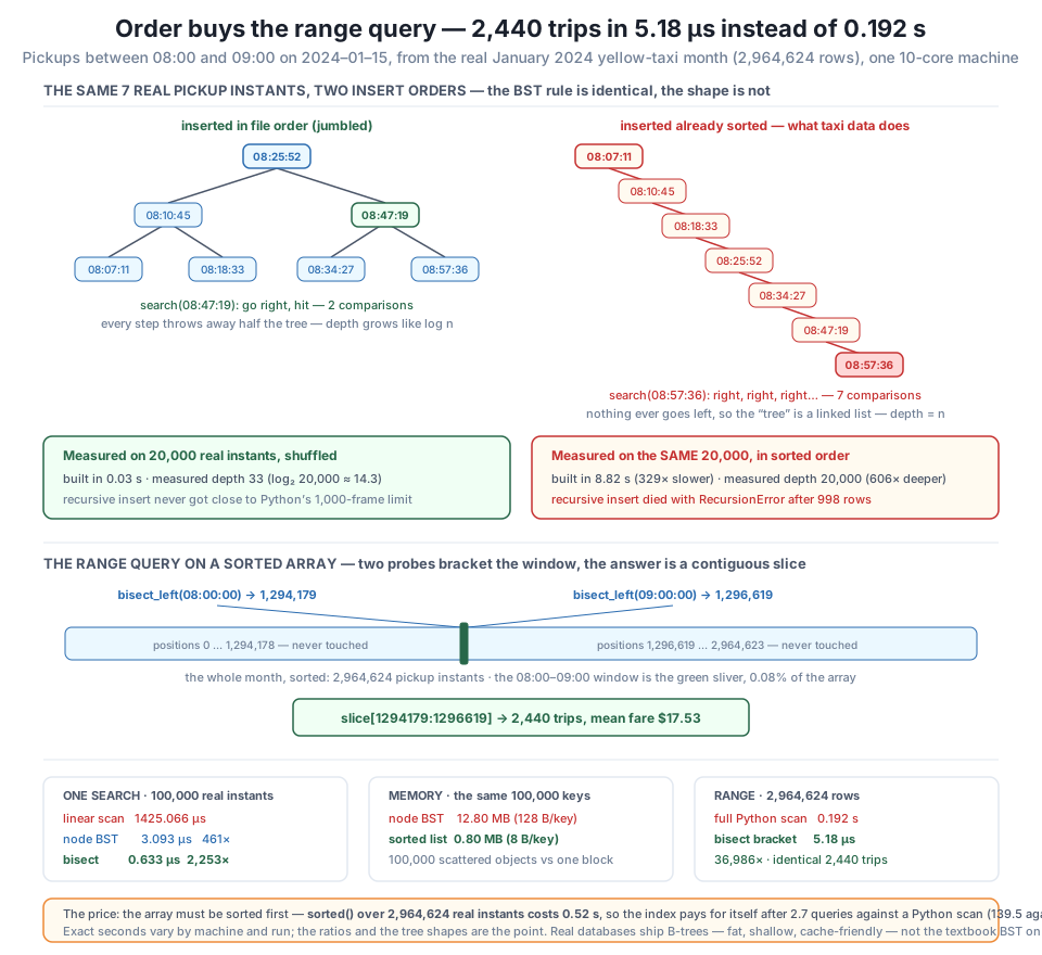
insert dies with a RecursionError after just 998 rows. Middle: two bisect_left probes bracket 08:00–09:00 on 2024–01–15 at positions 1,294,179 and 1,296,619, and the answer is the contiguous slice between them — 2,440 trips, 0.08% of the array, with 99.92% never touched. Bottom: the honest ranking over 100,000 real instants is linear scan 1425.066 µs, node BST 3.093 µs, bisect 0.633 µs per search — bisect beats the hand-rolled tree by 4.9× on 1/16th the memory, because contiguous C beats pointer-chasing Python. The range itself lands in 5.18 µs against a 0.192 s full scan (36,986×), bought with one 0.52 s sort. Exact seconds vary by machine and run; the ratios are the point.Everything so far has been about finding one key, and honestly, for one key the dict already won — 0.063 µs beats bisect’s 0.633 µs by 10x. Order does not exist to make exact lookups faster. It exists to make the question the dict cannot answer possible.
Sort the month first. This is the price, paid once, and we will look at the bill in a moment:
start = time.perf_counter()
sorted_pickups = sorted(pickup_us)
sort_secs = time.perf_counter() - start
print(f"sorted() over {len(pickup_us):,} real pickup instants: {sort_secs:.2f} s")
print(f"  first: {np.datetime64(sorted_pickups[0], 'us')}")
print(f"  last : {np.datetime64(sorted_pickups[-1], 'us')}")
sorted() over 2,964,624 real pickup instants: 0.52 s
first: 2002-12-31T22:59:39.000000
last : 2024-02-01T00:01:15.000000(There is that broken 2002 meter, sorted dutifully to position zero. Order is a property of the keys, not a judgement about them.)
Now the range query, twice — once by scanning all 2,964,624 rows, once with two bisect probes:
start = time.perf_counter()
scan_hits = 0
for k in pickup_us:
    if LO <= k < HI:
        scan_hits += 1
full_scan_secs = time.perf_counter() - start
print(f"full Python scan of {len(pickup_us):,} rows: {full_scan_secs:.3f} s -> {scan_hits:,} trips")

REPS = 1_000
start = time.perf_counter()
for _ in range(REPS):
    i = bisect.bisect_left(sorted_pickups, LO)
    j = bisect.bisect_left(sorted_pickups, HI)
    window = sorted_pickups[i:j]
bisect_range_secs = (time.perf_counter() - start) / REPS
print(f"bisect bracket + slice (avg of {REPS:,}): {bisect_range_secs * 1e6:.2f} us -> {len(window):,} trips")
print(f"  bisect_left(08:00) -> position {i:,}")
print(f"  bisect_left(09:00) -> position {j:,}")
print(f"  same answer as the scan: {len(window) == scan_hits}")
print(f"  {full_scan_secs / bisect_range_secs:,.0f}x faster")
full Python scan of 2,964,624 rows: 0.192 s -> 2,440 trips
bisect bracket + slice (avg of 1,000): 5.18 us -> 2,440 trips
bisect_left(08:00) -> position 1,294,179
bisect_left(09:00) -> position 1,296,619
same answer as the scan: True
36,986x faster5.18 µs against 0.192 s. Identical answer. 36,986x.
Look at what those two positions mean. bisect_left(sorted_pickups, LO) said 1,294,179: if 08:00:00 were in this array, it would go at index 1,294,179 — and because the array is sorted, everything before that index is earlier than 08:00 and cannot be in your window. bisect_left(sorted_pickups, HI) said 1,296,619: everything from there on is 09:00 or later. The answer is not “the rows that pass a test.” The answer is the rows between two numbers — sorted_pickups[1294179:1296619], a contiguous run of 2,440 items that the structure hands you without examining a single one of them.
That is the difference in kind, not degree. The scan touched all 2,964,624 keys and asked each one a question. bisect did about 22 comparisons — \( \log_2 \) of 2.96 million — twice, and then took a slice. 99.92% of the array was never looked at, and it never will be, no matter how many times you ask. That is what an index is, and CityFlow’s dashboard just became possible.
Use bisect_right when you want an inclusive upper bound: bisect_left(a, x) gives the position before any equal keys and bisect_right(a, x) the position after them, so a[bisect_left(a, lo):bisect_right(a, hi)] is the closed interval [lo, hi], while the bisect_left/bisect_left pair above is the half-open [lo, hi) that time windows almost always want. On 1,575,706 distinct instants shared by 2.96M trips, that boundary choice moves real rows.
A 36,986x that costs nothing would be a lie, so let’s find the cost. There are two, and the second one is the interesting one.
The first is the sort: 0.52 s. Against a 0.192 s scan, that means one query is a loss — you would have been faster just scanning. The index only wins if you ask more than once.
The second cost is subtler and it is why the honest opponent is not that Python loop. A pure-Python scan over three million rows is a straw man; nobody at CityFlow would write it when NumPy will do it vectorised, in C, on contiguous memory. And there is a second problem: sorted_pickups answers how many trips and which instants, but it has thrown away which rows — sorting the keys destroyed their alignment with the fare column. A real index has to carry the row positions along. np.argsort does exactly that: it returns the permutation that sorts the array, which you then apply to every column you want to keep aligned.
Build it properly and fight the real opponent:
keys_arr = np.asarray(pickup_us, dtype="int64")
fares_arr = trips["fare_amount"].to_numpy()

REPS = 20
start = time.perf_counter()
for _ in range(REPS):
    mask = (keys_arr >= LO) & (keys_arr < HI)
    scan_fares = fares_arr[mask]
    scan_mean = scan_fares.mean()
np_scan_secs = (time.perf_counter() - start) / REPS

start = time.perf_counter()
order = np.argsort(keys_arr, kind="stable")
sorted_keys_arr = keys_arr[order]
sorted_fares_arr = fares_arr[order]
index_build_secs = time.perf_counter() - start

REPS = 200
start = time.perf_counter()
for _ in range(REPS):
    a = np.searchsorted(sorted_keys_arr, LO, side="left")
    b = np.searchsorted(sorted_keys_arr, HI, side="left")
    idx_fares = sorted_fares_arr[a:b]
    idx_mean = idx_fares.mean()
np_index_secs = (time.perf_counter() - start) / REPS

print(f"index build (argsort + reorder keys and fares): {index_build_secs:.2f} s  (once)")
print(f"{'method':22s} {'per query':>12s} {'trips':>8s} {'mean fare':>11s}")
print(f"{'numpy full scan':22s} {np_scan_secs * 1000:10.2f} ms {len(scan_fares):8,} {scan_mean:10.2f}")
print(f"{'searchsorted + slice':22s} {np_index_secs * 1e6:10.2f} us {len(idx_fares):8,} {idx_mean:10.2f}")
print(f"identical answer: {abs(scan_mean - idx_mean) < 1e-9}")
print(f"speedup per query : {np_scan_secs / np_index_secs:,.0f}x")

saving = np_scan_secs - np_index_secs
print(f"saving per query  : {saving * 1000:.2f} ms")
print(f"crossover vs numpy scan : {index_build_secs / saving:.1f} queries")
py_saving = full_scan_secs - bisect_range_secs
print(f"crossover vs Python scan: {sort_secs / py_saving:.1f} queries")
index build (argsort + reorder keys and fares): 0.29 s (once)
method per query trips mean fare
numpy full scan 2.07 ms 2,440 17.53
searchsorted + slice 5.50 us 2,440 17.53
identical answer: True
speedup per query : 377x
saving per query : 2.07 ms
crossover vs numpy scan : 139.5 queries
crossover vs Python scan: 2.7 queriesnp.searchsorted is bisect for NumPy arrays — same binary search, same two probes — and because the fares were reordered by the same permutation at build time, sorted_fares_arr[a:b] is a contiguous slice of the right rows. CityFlow’s answer, for real: 2,440 trips between 08:00 and 09:00 on 15 January, mean fare \$17.53, in 5.50 µs.
And now the honest crossover, which is the number an engineer actually needs:
Both numbers are true and neither is the answer on its own. The answer depends on what CityFlow is building. A one-off analysis that asks “what happened between 8 and 9 on the 15th?” once should just scan — building the index would be pure loss. A dashboard — which is what this course has been building all along — asks that question every time somebody moves a date slider, for every hour, for every zone, thousands of times a day. At that volume 139.5 queries is the first ten seconds of the morning, and every query after it is 377x cheaper. That is the shape of every index decision you will ever make, and it is the same crossover logic Module 6 measured for the zone dict at 4.4 queries. Lesson 4 formalises it and Lesson 5 builds the artifact.
A sorted key column is only half an index
sorted(pickup_us) feels like an index and is not one. It can tell you how many trips fall in a window and what instants they started at, but the moment you sort the keys you break their correspondence with every other column — the fares, the zones, the distances. The bracket returns positions in the sorted array, which are meaningless to the original DataFrame. The fix is the one above: sort a permutation (np.argsort) rather than the keys alone, then apply that same permutation to every column you intend to read. Get this wrong and nothing raises an error; you just report the mean fare of 2,440 arbitrary trips with total confidence. Lesson 5 packages the whole thing so you cannot get it wrong twice.
Exercise 1 — Watch the depth grow with \( \log n \). The lesson measured one tree: 100,000 shuffled keys, depth 45. Test the claim that depth grows logarithmically by building shuffled BSTs over 1,000, 10,000, and 100,000 real distinct instants and printing the measured depth beside \( \log_2 n \) for each. The input grows 100x across the series — does the depth? Then repeat the whole series with sorted input (use insert_iter, and keep n small enough to finish) and print that depth column too. Describe both shapes in a comment.
Hint
Reuse max_depth — it is iterative for exactly this reason, and a recursive version would die on the sorted series. Expect the shuffled depths to land somewhere around \( 1.4 \times \log_2 n \) rather than exactly on it; random insertion buys you the right shape, not the ideal constant. The sorted series needs no measurement to predict — depth will equal n every time — but seeing the build time explode as you go from 5,000 to 20,000 is the real payoff, because it is quadratic, not linear.
Exercise 2 — Bracket a busier window, and check your boundaries. The lesson pulled 08:00–09:00 on 15 January: 2,440 trips. Use bisect_left and bisect_right over sorted_pickups to answer three more questions on the real month: how many trips started between 17:00 and 18:00 on the same day, how many started in the whole of 15 January, and how many started in the first minute of the month. Then do the last one twice — once with the half-open [lo, hi) bracket and once with the closed [lo, hi] bracket — and explain the difference in the counts.
Hint
Build your bounds with int(np.datetime64("2024-01-15T17:00:00", "us").astype("int64")) so the unit always matches the keys. The half-open versus closed difference will be exactly the number of trips whose pickup instant equals hi — small, but not zero on a dataset where 1,575,706 distinct instants are shared by 2,964,624 trips. That is the kind of off-by-one that produces a dashboard where consecutive hourly buckets do not add up to the daily total.
Exercise 3 — Find the real crossover for your query pattern. The lesson reported two crossovers — 2.7 queries against a Python scan, 139.5 against a NumPy one — because the answer depends entirely on the opponent. Now find it for a pattern CityFlow actually has. Write a function total_cost(n_queries, use_index) that measures the whole cost of answering n_queries random one-hour windows: the index build plus n_queries bracketed lookups, versus n_queries NumPy scans with no build. Run it for n_queries in (1, 10, 100, 1_000) and print both totals side by side. At what count does the index win, and how close is it to the lesson’s 139.5?
Hint
Draw your random windows from real timestamps so the answers are real — pick a random hour of a random day in January. The index build must be inside the timed region for the index version; that is the entire point. Expect your crossover to sit near, but not exactly on, the lesson’s number, because the cost of a bracket depends slightly on how many rows the window returns (the slice has to be materialised) and 08:00–09:00 is a busy hour. Note in a comment what happens to the crossover if the query set is bigger — and what that implies about whether “should I index?” has an answer that does not mention the query pattern.
You found the dict’s edge and bought your way past it. A hash table answers exact match in 0.063 µs and cannot answer a range query at all — measured on the real month, pickups one second apart land in slots 360,448 and 1,360,448 of a 4,194,304-slot table, so the only route to “trips between 08:00 and 09:00” is to examine all 1,575,706 keys, which costs 0.141 s and makes the dict worse than useless. What a range needs is order. A binary search tree keeps it: every left subtree smaller, every right subtree larger, so each comparison discards half the candidates — over 100,000 real instants that is a measured depth of 45 against a linear scan’s 100,000, and reading the tree in-order returns the keys sorted without sorting anything. But the textbook BST has a failure mode that taxi data walks straight into: fed already-sorted keys, the recursive insert died with a RecursionError after 998 rows, and the iterative version built a 20,000-deep linked list out of 20,000 nodes in 8.82 s — 329x slower and 606x deeper than the same keys shuffled (0.03 s, depth 33). And even at its best, the hand-rolled tree loses: over 100,000 real instants, a linear scan costs 1425.066 µs per search, the node BST 3.093 µs, and bisect on a sorted list 0.633 µs — bisect beats the tree by 4.9x on 1/16th the memory (0.80 MB against 12.80 MB), because contiguous C beats pointer-chasing Python. Which is exactly why real databases ship cache-friendly B-trees, not textbook BSTs. The payoff is the range: bisect_left bracketed 08:00–09:00 on 15 January at positions 1,294,179 and 1,296,619, returning 2,440 trips in 5.18 µs against a 0.192 s full scan — 36,986x, with 99.92% of the array never touched. The price is honest: sorted() over 2,964,624 instants costs 0.52 s, a properly aligned np.argsort index costs 0.29 s, and the crossover is 2.7 queries against a Python scan or 139.5 against a NumPy vectorised one — worth it for a dashboard, a waste for a one-off.
RecursionError after 998 recursive inserts. Balance is a lucky consequence of insertion order, not a property of the structure — and timestamps never arrive lucky.bisect on a sorted array — the practical BST in Python. Identical halving, but the tree is implicit in the index arithmetic, so there are no node objects, no pointer chasing, and no cache misses: 0.633 µs against the hand-rolled tree’s 3.093 µs (4.9x) on 8 bytes per key against 128 (16x). B-trees are this insight applied inside real databases.np.argsort index. That build amortises after 2.7 queries against a Python scan and 139.5 against a NumPy one, so “should I index?” is never answerable without knowing how many times you will ask.CityFlow’s dashboard needs one thing this pipeline could not do: ask for a slice of time. Every structure the course built before this lesson answers a different question — the loader answers “give me the data,” the parallel aggregation answers “summarise all of it,” the zone dict answers “what is id 132.” None of them can answer “what happened between 8 and 9,” and the fastest of them is the least capable of it, because the \( O(1) \) came from destroying order. That trade is the most important idea in this module: every structure buys a capability by giving one up, and knowing what you gave up is the whole job. The BST buys the range back, and measuring it honestly taught two things that a textbook would not. The first is that the idea — halve the candidates at every comparison — is worth 2,253x over a scan and is completely sound. The second is that the implementation everyone teaches is the wrong one for Python: the hand-rolled tree lost to twenty lines of bisect by 4.9x on a sixteenth of the memory, and would have taken the ingest down with a RecursionError on row 998 of ordinary, correctly-sorted input. An engineer who learned only the concept would have shipped that tree. An engineer who measured it ships the sorted array, understands why B-trees exist when they meet one in Lesson 4, and can say out loud what the index costs: 0.29 s up front, break-even at 139.5 queries, 377x forever after. That last sentence — the honest price, not just the headline speedup — is what separates a fast answer from a defensible one.
Sorting bought you everything in this lesson, and that quiet 0.52 s assumed something the rest of this course has spent five modules refusing to assume: that the whole month fits in memory at once. It does here — 2.96 million integers is a manageable 23 MB — but Module 4 dealt with files that do not fit, and sorted() has no answer for those. Lesson 3, Trees for Sorting & Merging, closes that gap with the technique that has been solving it since tape drives: sort the chunks that do fit, then merge the sorted runs into one ordered stream without ever holding more than one row from each. You’ll meet heapq.merge, which is Module 6’s heap doing a job you have not seen it do — k-way merging, where the heap holds one candidate per input run and always knows which is smallest next — and you’ll build an external sort that produces the same sorted key array this lesson depended on, over data far larger than RAM. It is the moment Module 4’s chunking and Module 6’s heaps turn out to have been the same lesson all along, and it is the last piece CityFlow needs before Lesson 4 turns a sorted key array into a real file index.
Keep DATATWEETS free. Help fund practical data, AI, and engineering lessons for learners worldwide.
