Title here
Summary here
Two of this course’s threads have been running in parallel, and this is the lesson where they meet. Module 4 taught CityFlow’s pipeline to chunk: when the month does not fit, read it in pieces, do the work piece by piece, and never let the whole thing land in RAM at once. Module 6 taught the heap: a tree flattened into a plain Python list, whose one talent is producing the smallest item of a collection on demand for \( O(\log n) \). Each was useful alone. Together they answer a question that neither can touch by itself: how do you sort data that does not fit in memory?
That question is not academic, and it is not rare. sorted() is the most casually-typed function in Python and it has one absolute requirement — the entire list has to be in RAM, because Timsort needs random access to every element to move it around. Sorting January 2024’s 2,964,624 pickup timestamps that way peaks at 166.1 MB, which this machine shrugs off. Ask for a year and it is 2 GB; ask for the decade the TLC actually publishes and sorted() is not slow, it is impossible. This lesson builds the way out, and it is the single most important out-of-core algorithm in data engineering: external sorting. You cannot sort three million timestamps at once, but you can sort 250,000 of them twelve times and then merge the results — and merging, it turns out, needs almost no memory at all. You will hand-roll the two-run merge, discover that merging k runs is precisely the question a heap exists to answer, and then run the whole thing for real on the month: 12 sorted runs written to actual files, streamed back through heapq.merge, producing output byte-for-byte identical to sorted() while peaking at 22.1 MB — 7.5x less. It will also be 2.7x slower, and we are going to say so plainly, because like Module 6’s bounded heap this trade buys capability, not speed.
By the end of this lesson, you will be able to:
heapq.merge and understand exactly what it is doing lazily on your behalfsorted() already does with pre-sorted runsYou’ll need pandas, numpy, and Python’s standard library (heapq, array, tracemalloc). Let’s sort something that doesn’t fit.
The data is the public NYC TLC Trip Record Data — the same January 2024 yellow-taxi month the whole course has used. Fetch it once and keep it beside your script:
# gate: skip
# CityFlow's month of trips, fetched once from the public TLC mirror.
import urllib.request
urllib.request.urlretrieve(
    "https://d37ci6vzurychx.cloudfront.net/trip-data/yellow_tripdata_2024-01.parquet",
    "yellow_tripdata_2024-01.parquet",
)
External sort is an algorithm about files, so we start by making one. Pull the pickup timestamps out of the parquet and write them to a flat file of fixed-width records — 8 bytes per timestamp, microseconds since the epoch, nothing else. This is deliberately the least clever file format imaginable, and that is the point: a record file you can read a chunk at a time, seek around in, and reason about exactly. It is also what a database’s sort spill actually looks like.
Everything this lesson writes goes into one private spill directory from tempfile.mkdtemp(). That is not housekeeping pedantry — an external sort’s whole method is leaving intermediate files lying around, and two copies of this pipeline running at once with hard-coded filenames would silently overwrite each other’s runs and produce wrong output, quietly. A unique directory per run makes that impossible, and it makes cleanup a single rmtree at the end. We pass dir="." to keep the spill beside the data; in production this is the one knob you do want configurable, pointed at whichever volume has room and speed to spare.
import warnings
warnings.filterwarnings("ignore")
import pandas as pd
import numpy as np
import heapq
import time
import os
import gc
import sys
import math
import random
import shutil
import tempfile
import tracemalloc
from array import array

SPILL = tempfile.mkdtemp(prefix="external_sort_", dir=".")
SRC = os.path.join(SPILL, "pickup_us.bin")

t0 = time.perf_counter()
pickups = pd.read_parquet(
    "yellow_tripdata_2024-01.parquet", columns=["tpep_pickup_datetime"]
)["tpep_pickup_datetime"]
stamps = array("q", pickups.astype("int64").tolist())
with open(SRC, "wb") as f:
    stamps.tofile(f)
print(f"extracted {len(stamps):,} pickup timestamps in {time.perf_counter() - t0:.2f} s")
print(f"pickup_us.bin on disk: {os.path.getsize(SRC) / 1e6:.2f} MB "
      f"({os.path.getsize(SRC) // len(stamps)} bytes per record)")
print("first three records:", list(stamps[:3]))
print("as timestamps      :", [str(pd.Timestamp(v, unit='us')) for v in stamps[:3]])
del pickups, stamps
gc.collect()
extracted 2,964,624 pickup timestamps in 0.35 s
pickup_us.bin on disk: 23.72 MB (8 bytes per record)
first three records: [1704070675000000, 1704067380000000, 1704068226000000]
as timestamps : ['2024-01-01 00:57:55', '2024-01-01 00:03:00', '2024-01-01 00:17:06']23.72 MB on disk for the whole column: 2,964,624 records at 8 bytes each, and not a byte of overhead. Hold that number, because it is about to be the most interesting comparison in the lesson. Note the first three records too — 00:57:55 followed by 00:03:00 followed by 00:17:06. The file is not sorted.
Now do the obvious thing. Read it all in and sort it:
def read_all(path):
    """Load an entire run file into a Python list of ints."""
    values = array("q")
    with open(path, "rb") as f:
        values.fromfile(f, os.path.getsize(path) // 8)
    return values.tolist()

t = time.perf_counter()
vals = read_all(SRC)
read_secs = time.perf_counter() - t

t = time.perf_counter()
ref = sorted(vals)
sort_secs = time.perf_counter() - t

print(f"read  {len(vals):,} timestamps into a list : {read_secs:.2f} s")
print(f"sorted() the whole list                  : {sort_secs:.2f} s")
print(f"earliest pickup: {pd.Timestamp(ref[0], unit='us')}")
print(f"latest pickup  : {pd.Timestamp(ref[-1], unit='us')}")
print(f"list container alone: {sys.getsizeof(ref) / 1e6:.2f} MB "
      f"(pointers only, not the {len(ref):,} int objects they point at)")
read 2,964,624 timestamps into a list : 0.06 s
sorted() the whole list : 0.51 s
earliest pickup: 2002-12-31 22:59:39
latest pickup : 2024-02-01 00:01:15
list container alone: 23.72 MB (pointers only, not the 2,964,624 int objects they point at)Half a second. sorted() is superb and there is nothing wrong with this code — at this size. But look at what it needed to do it, and notice the honest accounting problem hiding in that last line. The list container is 23.72 MB, which looks reassuringly like the file — but that is 2,964,624 pointers at 8 bytes each, and every one of them points at a Python int object costing another 28-32 bytes. sys.getsizeof on the list reports the pointer array and stops there. The real bill is several times larger, and we will measure it properly with tracemalloc later in the lesson rather than estimate it now.
(The sorted extremes are a free data-quality finding, and a preview of Lesson 4: the earliest “January 2024” pickup is 2002-12-31 22:59:39 and the latest is 2024-02-01 00:01:15. Both are outside the month. This is the same dirt Module 3 found in trip_distance, and it is worth noticing how we found it — sorting a column puts its worst values at the two ends where you cannot miss them.)
Here is the question that makes this lesson necessary. sorted() needs the whole list in RAM because Timsort moves elements around by index; there is no way to sort by index into something you have not loaded. So what happens when the data is 10x this? 100x? At some point read_all raises MemoryError and the pipeline stops — not slowly, just stops. Adding cores does not help; Module 5’s ten processes each need the data too. You cannot sort it at once. But you can sort pieces of it, and then combine the pieces. That second half is where all the leverage is, and it rests on one small, beautiful primitive.
A run is just a sorted sequence. The claim is this: given two runs, you can produce one correctly-sorted run containing both, and the only thing you ever need to look at is the first element of each.
Think about why that is true, because the reason is the whole lesson. If run A is sorted, then A[0] is the smallest thing in A — nothing later in A can beat it. Same for B[0] and B. So the smallest thing in both runs must be one of those two, and you can settle it with a single comparison. Take the winner, advance that run by one, and now the same argument applies again to what remains. Repeat until both are empty. You never look ahead, you never look back, you never need the runs to be in memory — you only need to be able to ask each one “what’s next?”
def merge_two(a, b):
    """Merge two already-sorted lists. Holds one element from each at a time."""
    out = []
    i = j = 0
    while i < len(a) and j < len(b):
        if a[i] <= b[j]:
            out.append(a[i])
            i += 1
        else:
            out.append(b[j])
            j += 1
    out.extend(a[i:])
    out.extend(b[j:])
    return out

demo_a = sorted(vals[:6])
demo_b = sorted(vals[6:12])
print("run A (sorted):", [str(pd.Timestamp(v, unit='us').time()) for v in demo_a])
print("run B (sorted):", [str(pd.Timestamp(v, unit='us').time()) for v in demo_b])
print("merged        :", [str(pd.Timestamp(v, unit='us').time()) for v in merge_two(demo_a, demo_b)])

CHUNK = 250_000
run_a = sorted(vals[:CHUNK])
run_b = sorted(vals[CHUNK:2 * CHUNK])
t = time.perf_counter()
merged = merge_two(run_a, run_b)
merge_two_secs = time.perf_counter() - t
print(f"\nmerge_two on {len(run_a):,} + {len(run_b):,} real timestamps: {merge_two_secs:.3f} s")
print(f"  result length          : {len(merged):,}")
print(f"  identical to sorted()  : {merged == sorted(vals[:2 * CHUNK])}")
print(f"  cost per element       : {merge_two_secs / len(merged) * 1e9:.0f} ns")
run A (sorted): ['00:03:00', '00:17:06', '00:36:38', '00:46:51', '00:54:08', '00:57:55']
run B (sorted): ['00:25:00', '00:26:01', '00:28:08', '00:30:40', '00:35:22', '00:49:44']
merged : ['00:03:00', '00:17:06', '00:25:00', '00:26:01', '00:28:08', '00:30:40', '00:35:22', '00:36:38', '00:46:51', '00:49:44', '00:54:08', '00:57:55']
merge_two on 250,000 + 250,000 real timestamps: 0.041 s
result length : 500,000
identical to sorted() : True
cost per element : 82 nsTwo properties, both essential.
First, it is correct, and not by luck — the merged output is identical to what sorted() produces on the same 500,000 real timestamps. Follow the small demo by eye: the merged line interleaves the two runs exactly where it should, taking 00:03:00 and 00:17:06 from A, then four in a row from B, then back to A. Nothing sophisticated happened. It kept taking the smaller head.
Second, it is \( O(n) \) — linear, not \( n \log n \). Each loop iteration does one comparison and permanently consumes one element, so the total work is exactly the number of elements. At 82 nanoseconds per element on real data, merging is cheaper than sorting, and that asymmetry is what the rest of the lesson spends. Sorting is the expensive thing you do to small pieces; merging is the cheap thing you do to big ones.
And now the property that matters most, the one you have to squint to see because our version does not exploit it yet: merge_two touched a[i] and b[j] and nothing else. It never needed a[500] while looking at a[3]. Both lists happen to be in memory here, but the algorithm never asked for that. Replace a and b with anything that can produce values one at a time — a generator, an open file, a network socket — and the merge works unchanged, with two elements in RAM instead of half a million. That is the door out of memory, and everything else here is walking through it.
Two runs is a warm-up. A real external sort produces a dozen runs, or a thousand, and merging them pairwise — merge 1 and 2, merge that with 3, merge that with 4 — works but rereads the accumulating output on every pass, which is \( O(nk) \) and wasteful. You want to merge all k at once, in a single pass.
Restate the merge rule for k runs and the problem announces itself: repeatedly take the smallest of the k heads. Which means, three million times over, you need the answer to one question — which of these k values is smallest, and which run did it come from? — with the wrinkle that after each answer, one head changes and you have to ask again.
That is not a new problem. That is the exact problem Module 6 solved. A heap is a binary tree with one rule — every node is smaller than both its children — which forces the global minimum to sit at the root where you can read it for free, and lets you restore the rule after a change by walking a single root-to-leaf path. Push, pop, and re-heapify all cost \( O(\log k) \) because the tree’s height is \( \log_2 k \). A structure whose entire purpose is “hand me the smallest, repeatedly, as the contents change” is not merely usable for k-way merging — it is a description of k-way merging.
So: put one (head_value, run_index) pair per run into a heap. Pop the root — that is the next output value, globally. Pull the next value from that run only and push it. Repeat.
runs = [sorted(vals[i:i + CHUNK]) for i in range(0, len(vals), CHUNK)]
print(f"k = {len(runs)} sorted runs, sizes: {[len(r) for r in runs[:3]]} ... {len(runs[-1]):,}")

def kway_merge(runs):
    """Merge k sorted runs using a heap of the k current heads."""
    heap = []
    cursors = [iter(r) for r in runs]
    for idx, cur in enumerate(cursors):
        try:
            heap.append((next(cur), idx))
        except StopIteration:
            pass
    heapq.heapify(heap)
    while heap:
        value, idx = heapq.heappop(heap)
        yield value
        try:
            heapq.heappush(heap, (next(cursors[idx]), idx))
        except StopIteration:
            pass

t = time.perf_counter()
hand = list(kway_merge(runs))
hand_secs = time.perf_counter() - t

t = time.perf_counter()
lib = list(heapq.merge(*runs))
lib_secs = time.perf_counter() - t

print(f"\nhand-rolled heap k-way merge : {hand_secs:.2f} s   matches sorted(): {hand == ref}")
print(f"heapq.merge(*runs)           : {lib_secs:.2f} s   matches sorted(): {lib == ref}")
print(f"heap holds {len(runs)} items; log2({len(runs)}) = {math.log2(len(runs)):.2f} comparisons per element")
del hand, lib
gc.collect()
k = 12 sorted runs, sizes: [250000, 250000, 250000] ... 214,624
hand-rolled heap k-way merge : 0.65 s matches sorted(): True
heapq.merge(*runs) : 0.50 s matches sorted(): True
heap holds 12 items; log2(12) = 3.58 comparisons per elementBoth reproduce sorted() exactly across all 2,964,624 timestamps. The 25 lines of kway_merge and the one line of heapq.merge(*runs) are the same algorithm; the standard library’s version is a little faster (0.50 s vs 0.65 s) because it is written by people who have optimised it for twenty years, and it is the one you should use. Write the hand-rolled one once, to know what you are calling.
heapq.merge deserves a closer look, because its two properties are exactly the two we need. It takes iterables, not lists — anything that produces values in order. And it returns a lazy iterator: nothing is merged until you ask, and asking for one value pulls one value. That combination is why it can merge inputs that would never fit together in RAM.
Now, is the heap actually earning its keep? At k=12 you could just check all twelve heads with a for loop. Let’s measure that honestly, sweeping k:
def kway_scan(runs):
    """Same merge, but find the smallest head by checking all k of them."""
    pos = [0] * len(runs)
    remaining = sum(len(r) for r in runs)
    while remaining:
        best = None
        best_i = -1
        for i, run in enumerate(runs):
            if pos[i] < len(run):
                v = run[pos[i]]
                if best is None or v < best:
                    best = v
                    best_i = i
        pos[best_i] += 1
        remaining -= 1
        yield best

sample = vals[:600_000]
sample_ref = sorted(sample)
print(f"merging {len(sample):,} real timestamps, split k ways\n")
print(f"{'k runs':>7} {'heap O(log k)':>15} {'scan O(k)':>12} {'scan/heap':>11}")
for k in (4, 12, 64, 256):
    size = (len(sample) + k - 1) // k
    parts = [sorted(sample[i:i + size]) for i in range(0, len(sample), size)]
    t = time.perf_counter()
    by_heap = list(kway_merge(parts))
    heap_secs = time.perf_counter() - t
    t = time.perf_counter()
    by_scan = list(kway_scan(parts))
    scan_secs = time.perf_counter() - t
    assert by_heap == sample_ref and by_scan == sample_ref
    print(f"{len(parts):7d} {heap_secs:14.2f}s {scan_secs:11.2f}s {scan_secs / heap_secs:10.1f}x")
del sample, sample_ref
gc.collect()
merging 600,000 real timestamps, split k ways
k runs heap O(log k) scan O(k) scan/heap
4 0.10s 0.35s 3.5x
12 0.13s 0.54s 4.0x
64 0.19s 2.30s 11.8x
256 0.25s 8.48s 33.9xRead the two middle columns as sequences rather than as four separate races, because the shapes are the finding. The scan column quadruples every time k quadruples — 0.35, 0.54, 2.30, 8.48. The first step understates it (0.35 s at k=4 is a noisy measurement of a fast loop), but from k=12 onward it is unmistakable. It grows that way because checking k heads costs k, and the same 600,000 elements each pay it. That is \( O(k) \) per element, doing about 256 comparisons per output value at the right-hand end.
The heap column barely moves: 0.10, 0.13, 0.19, 0.25. Sixty-four times as many runs cost 2.5x more time, because the heap’s cost is the height of the tree, and \( \log_2 4 = 2 \) while \( \log_2 256 = 8 \) — four times the height for sixty-four times the runs. That is what a logarithm buys, and it is why the answer to “how many runs can I merge at once?” is “more than you were planning to.”
Note the honest reading at k=4: 3.5x. At small k the heap wins something, but not something you would restructure code for — the same shape Module 6 found when a bounded heap beat sorted() by only 1.65x on 260 zones. The heap is not magic at small scale. It becomes indispensable as k grows, which is precisely the direction external sorting pushes k: the less RAM you have, the smaller your chunks, the more runs you get.
Now assemble it. The algorithm is two phases and the whole thing is about twenty lines.
Phase 1, sort: read the input in chunks that comfortably fit, sort each chunk with sorted() (using the fast, in-memory algorithm on a piece where it is legal), and write each sorted chunk to its own file. These files are the runs. RAM held: one chunk.
Phase 2, merge: open all the runs, stream them through heapq.merge, and write the merged output as it comes. RAM held: one small buffer per run, plus the heap of k heads.
The critical detail is that the readers must be generators. A function that returns a list has already lost — it read the whole run into memory, which is the thing we are avoiding. stream_run below reads 8,192 records at a time and yields them one by one, so it holds 64 KB regardless of whether the run is 2 MB or 2 TB.
def read_chunks(path, chunk_rows):
    """Yield successive lists of at most chunk_rows values from a record file."""
    with open(path, "rb") as f:
        while True:
            buf = array("q")
            try:
                buf.fromfile(f, chunk_rows)
            except EOFError:
                pass
            if not buf:
                return
            yield buf.tolist()

def stream_run(path, buf_rows=8192):
    """Yield values from a sorted run file, holding only buf_rows at a time."""
    with open(path, "rb") as f:
        while True:
            buf = array("q")
            try:
                buf.fromfile(f, buf_rows)
            except EOFError:
                pass
            if not buf:
                return
            yield from buf

def external_sort(src, dst, chunk_rows=250_000, out_buf=65_536):
    run_paths = []
    for i, chunk in enumerate(read_chunks(src, chunk_rows)):
        chunk.sort()
        path = os.path.join(SPILL, f"run_{i:02d}.bin")
        with open(path, "wb") as f:
            array("q", chunk).tofile(f)
        run_paths.append(path)
        del chunk
    with open(dst, "wb") as f:
        buf = array("q")
        for value in heapq.merge(*[stream_run(p) for p in run_paths]):
            buf.append(value)
            if len(buf) >= out_buf:
                buf.tofile(f)
                buf = array("q")
        if buf:
            buf.tofile(f)
    return run_paths

DST = os.path.join(SPILL, "sorted_out.bin")

t = time.perf_counter()
run_files = external_sort(SRC, DST)
external_secs = time.perf_counter() - t

print(f"external sort wrote {len(run_files)} runs and merged them in {external_secs:.2f} s")
print(f"  run files on disk : {sum(os.path.getsize(p) for p in run_files) / 1e6:.2f} MB")
print(f"  output on disk    : {os.path.getsize(DST) / 1e6:.2f} MB")
external_out = read_all(DST)
print(f"  identical to sorted(vals) : {external_out == ref}")
print(f"\nin-memory sorted()  : {read_secs + sort_secs:.2f} s (read {read_secs:.2f} + sort {sort_secs:.2f})")
print(f"external sort       : {external_secs:.2f} s  ({external_secs / (read_secs + sort_secs):.1f}x slower)")
del external_out
gc.collect()
external sort wrote 12 runs and merged them in 1.55 s
run files on disk : 23.72 MB
output on disk : 23.72 MB
identical to sorted(vals) : True
in-memory sorted() : 0.56 s (read 0.06 + sort 0.51)
external sort : 1.55 s (2.7x slower)It works. 2,964,624 timestamps, fully sorted, byte-for-byte identical to sorted() — produced by a process that never held more than 250,000 of them at a time. And it is 2.7x slower, 1.55 s against 0.56 s.
Say that out loud rather than bury it, because the temptation to present external sort as an optimisation is strong and it is a lie. It is slower, and it is obviously slower once you count what it does: it sorts the same data (in twelve pieces), then writes 23.72 MB to disk, then reads 23.72 MB back, then merges every element through a heap, then writes 23.72 MB out again. The in-memory version does none of that. External sort will never beat an in-memory sort on data that fits in memory, on any machine, ever.
This is precisely the shape of Module 6’s bounded heap, which turned out slower than nlargest and was worth having anyway. The external sort does not buy speed. It buys the ability to finish. Which brings us to the number this lesson is actually about.
Time was never the claim. Memory is. Measure both paths with tracemalloc, which counts every allocation Python’s own allocator makes inside the traced block and reports the high-water mark — so it sees our lists, ints, and array buffers precisely. Two honest limits worth stating: it does not count memory allocated inside C extensions (pandas and pyarrow live largely outside it), and it does not count the operating system’s file cache, which is why the external sort’s disk traffic is invisible here. Both paths in this comparison are pure Python objects read from a flat file, so the comparison is fair — but tracemalloc is not a process-memory monitor, and it also imposes serious overhead, which is why every timing above was taken with it switched off.
del runs, run_a, run_b, merged
gc.collect()

def in_memory_sort(src, dst):
    values = read_all(src)
    ordered = sorted(values)
    with open(dst, "wb") as f:
        array("q", ordered).tofile(f)

MEM_DST = os.path.join(SPILL, "mem_out.bin")

tracemalloc.start()
in_memory_sort(SRC, MEM_DST)
_, in_memory_peak = tracemalloc.get_traced_memory()
tracemalloc.stop()
gc.collect()

tracemalloc.start()
run_files = external_sort(SRC, DST)
_, external_peak = tracemalloc.get_traced_memory()
tracemalloc.stop()
gc.collect()

print(f"peak traced memory, in-memory sorted() : {in_memory_peak / 1e6:8.1f} MB")
print(f"peak traced memory, external sort      : {external_peak / 1e6:8.1f} MB")
print(f"the external sort holds {in_memory_peak / external_peak:.1f}x less")
same = read_all(MEM_DST) == read_all(DST)
print(f"byte-for-byte same answer              : {same}")
peak traced memory, in-memory sorted() : 166.1 MB
peak traced memory, external sort : 22.1 MB
the external sort holds 7.5x less
byte-for-byte same answer : True166.1 MB against 22.1 MB, for the identical answer. That is the lesson.
Both halves of that are worth unpacking. The in-memory sort’s 166.1 MB is the honest price of a file that is 23.72 MB on disk — a 7x inflation that has nothing to do with sorting and everything to do with Python. Each 8-byte record becomes an int object of roughly 32 bytes, plus 8 bytes for the list pointer, and then sorted() allocates a second list to return. This is the tax Module 1 introduced and Module 2 escaped with NumPy; here it means “my data is only 24 MB” and “I need 166 MB to sort it” are both true at once.
The external sort’s 22.1 MB is set by something completely different: the chunk size you chose. 250,000 records inflate to about 11 MB of Python ints, doubled while array("q", chunk) copies them out to disk, plus twelve 8,192-record read buffers during the merge. Nowhere in that sentence does the size of the input file appear. Sort ten times as much data with the same 250,000-row chunks and you get 120 runs instead of 12, the merge heap grows from 12 items to 120 (\( \log_2 120 = 6.9 \) comparisons instead of 3.58, so slightly slower), and the peak memory barely moves. The in-memory sort’s RAM is a function of the data. The external sort’s RAM is a function of your configuration. That is not a speedup; it is a different relationship with the problem, and it is why every database on earth sorts this way.
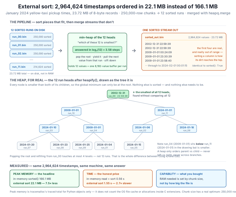
heapq.merge, holding one 8,192-value buffer per run. The middle panel is the actual heap after heapify() — 12 real run heads, four levels deep — and it shows the one rule a heap enforces: every node beats its children, so the global minimum is pinned at the root, while run_04's 2009-01-01 sits two levels below run_11's 2024-01-01 despite being smaller, because a heap never orders siblings. Popping the root costs \( \log_2 12 = 3.58 \) comparisons rather than a scan of all 12. The result: 22.1 MB peak against 166.1 MB for output byte-for-byte identical to sorted() — 7.5× less memory for 2.7× more time (1.55 s vs 0.56 s). External sort never wins on speed; it wins by making the RAM bill a function of your chunk size instead of your data size. Exact seconds vary by machine and run.So what is the right chunk size? There is a real optimum, and it is not “as small as possible” — the two phases pull in opposite directions. Sweep it:
print(f"{'chunk rows':>11} {'runs (k)':>9} {'peak MB':>9} {'run files MB':>13}")
for chunk_rows in (1_000_000, 250_000, 50_000, 10_000):
    gc.collect()
    tracemalloc.start()
    paths = external_sort(SRC, DST, chunk_rows=chunk_rows)
    _, peak = tracemalloc.get_traced_memory()
    tracemalloc.stop()
    on_disk = sum(os.path.getsize(p) for p in paths) / 1e6
    print(f"{chunk_rows:11,} {len(paths):9d} {peak / 1e6:9.1f} {on_disk:13.2f}")
    for p in paths:
        os.remove(p)
chunk rows runs (k) peak MB run files MB
1,000,000 3 88.5 23.72
250,000 12 22.1 23.72
50,000 60 5.0 23.72
10,000 297 22.5 23.72A U-shape, and an instructive one. Going from 1,000,000-row chunks to 50,000 cuts peak memory from 88.5 MB to 5.0 MB exactly as you would expect — smaller chunks, less RAM. Then 10,000-row chunks make it worse, back up to 22.5 MB, which looks like a bug and is not. Shrinking the chunk shrinks phase 1’s footprint but multiplies k, and phase 2 pays for k: 297 runs means 297 open files each holding an 8,192-record buffer, and those buffers now cost more than the sort chunk ever did. The disk footprint never budges — 23.72 MB of runs regardless, because it is the same data.
The rule of thumb: make chunks as large as your memory budget allows, not as small as you can manage. Bigger chunks mean fewer runs, a shorter heap, less merge overhead, and less disk seeking. You shrink the chunk to fit the budget, and not one row further.
The generator is the whole trick
heapq.merge gives you nothing if you hand it lists. heapq.merge(*[read_all(p) for p in run_paths]) is valid Python, produces the correct answer, and has already loaded every run into RAM before the merge starts — which is the exact thing external sorting exists to prevent. The memory win lives entirely in stream_run being a generator: it holds 8,192 records, yields them one at a time, and reads the next block only when asked. The same trap sits on the output side — accumulating results into a list and writing at the end rebuilds the 166 MB you just avoided. Write as you go. If any single line of your out-of-core pipeline can hold the whole dataset, your pipeline is an in-memory pipeline with extra steps.
Step back and look at what you built, because you have seen its shape before — in Lesson 1, as the canonical example of divide and conquer. Split the problem in half, solve each half, combine the solutions. Merge sort splits a list, sorts both halves recursively, and merges them with exactly the “take the smaller head” routine you wrote as merge_two.
External sort is merge sort with two substitutions. The recursion stops early — instead of splitting all the way down to single elements, it stops as soon as a piece fits in RAM and lets sorted() finish the job, because at that size Timsort is better than anything you would write. And the intermediate results live on disk rather than on the call stack. That is all. The divide step is read_chunks, the conquer step is chunk.sort(), and the combine step is heapq.merge. Lesson 1’s warning about Python’s recursion limit is why this version is a flat loop rather than a recursive function: 12 levels of recursion would be fine, but the algorithm has no need for a stack at all when the runs can just sit in a list.
Which leaves one loose end, and it is a good one. If merging is what makes sorted runs valuable, does sorted() itself know about runs? It does — Python’s Timsort is built around exactly this idea. It scans for naturally-occurring ascending sequences in your data, treats each as a free pre-made run, and merges them. On data that is already sorted, Timsort finds one giant run, verifies it, and stops. The received wisdom is that real-world data is often “nearly sorted” and that Timsort therefore gets a big discount on it. Real taxi timestamps ought to be a perfect example — trips get recorded roughly as they happen.
Let’s check, rather than assume.
run_count = 1
for i in range(1, len(vals)):
    if vals[i] < vals[i - 1]:
        run_count += 1
print(f"maximal ascending runs in the file as delivered : {run_count:,}")
print(f"  average run length                           : {len(vals) / run_count:.2f} values")

shuffled = vals[:]
random.seed(7)
random.shuffle(shuffled)
shuffled_runs = 1
for i in range(1, len(shuffled)):
    if shuffled[i] < shuffled[i - 1]:
        shuffled_runs += 1
print(f"  the same values shuffled                     : {shuffled_runs:,} runs, average {len(shuffled) / shuffled_runs:.2f}")

block = len(vals) // 10
print("\nmedian pickup time per tenth of the file, in file order:")
for i in range(10):
    med = sorted(vals[i * block:(i + 1) * block])[block // 2]
    print(f"  tenth {i}: {pd.Timestamp(med, unit='us')}")
maximal ascending runs in the file as delivered : 1,290,559
average run length : 2.30 values
the same values shuffled : 1,482,361 runs, average 2.00
median pickup time per tenth of the file, in file order:
tenth 0: 2024-01-03 07:02:33
tenth 1: 2024-01-06 10:42:48
tenth 2: 2024-01-09 21:49:56
tenth 3: 2024-01-12 23:41:38
tenth 4: 2024-01-16 13:28:19
tenth 5: 2024-01-19 13:37:23
tenth 6: 2024-01-22 18:11:13
tenth 7: 2024-01-25 19:11:30
tenth 8: 2024-01-28 16:50:32
tenth 9: 2024-01-30 16:29:10The received wisdom is wrong here, and the data is more interesting than the story. The file contains 1,290,559 ascending runs averaging 2.30 values each. A randomly shuffled list of the same values gives 1,482,361 runs averaging 2.00. Two-point-three versus two: at the resolution Timsort’s run detector works at, this file is barely distinguishable from random. It is emphatically not “nearly sorted.”
And yet look at the medians. Tenth by tenth, they climb steadily from January 3rd to January 30th, without a single reversal. The month is ordered — globally, unmistakably. Both facts are true simultaneously, and reconciling them tells you what the file actually is: trips were recorded in roughly chronological order at the scale of days, but within any local neighbourhood the timestamps are thoroughly jumbled, because dozens of vendors report in batches with their own lags. Zoom out and it is sorted. Zoom in to consecutive rows and it is noise.
So does Timsort get a discount or not? Only the clock can say:
shuffled_fresh = np.array(shuffled).tolist()

t = time.perf_counter()
sorted(vals)
file_order_secs = time.perf_counter() - t
t = time.perf_counter()
sorted(shuffled_fresh)
shuffled_secs = time.perf_counter() - t
t = time.perf_counter()
sorted(ref)
presorted_secs = time.perf_counter() - t
t = time.perf_counter()
sorted(shuffled)
reused_secs = time.perf_counter() - t

print(f"sorted(file order)          : {file_order_secs:.2f} s")
print(f"sorted(shuffled)            : {shuffled_secs:.2f} s   ({shuffled_secs / file_order_secs:.2f}x slower than file order)")
print(f"sorted(already sorted)      : {presorted_secs:.2f} s   ({file_order_secs / presorted_secs:.1f}x faster than file order)")
print(f"sorted(shuffled, same ints) : {reused_secs:.2f} s   <- same values, same order as above, old objects")
sorted(file order) : 0.50 s
sorted(shuffled) : 1.38 s (2.73x slower than file order)
sorted(already sorted) : 0.11 s (4.8x faster than file order)
sorted(shuffled, same ints) : 1.98 s <- same values, same order as above, old objectsIt does. Sorting the file in its delivered order takes 0.50 s; sorting the identical values shuffled takes 1.38 s — a real 2.73x discount from ordering that the run-length statistic completely failed to predict. And the fully-sorted case shows what run detection is worth when it does fire: 0.11 s, 4.8x faster than file order, because Timsort finds one run and is essentially done.
That fourth line is a measurement-hygiene warning aimed at you. shuffled and shuffled_fresh hold the same values in the same order — the only difference is that shuffled_fresh was rebuilt through NumPy, so its int objects were allocated in list order, while shuffled still points at the original objects scattered across the heap. Same algorithm, same comparisons, 0.60 s of difference purely in cache misses from chasing pointers. Had we timed only shuffled, we would have reported 4.0x and quietly folded a memory-layout artifact into a claim about Timsort. When you benchmark a sort, shuffling a list of objects measures two things at once.
So where does the genuine 2.73x come from, if not from long runs? Stop timing and count the actual comparisons — the one metric no cache effect can contaminate:
class Counted:
    """Wraps a value and counts every comparison sorted() asks for."""
    __slots__ = ("v",)
    comparisons = 0

    def __init__(self, v):
        self.v = v

    def __lt__(self, other):
        Counted.comparisons += 1
        return self.v < other.v

N = 200_000
subset = vals[:N]
subset_shuffled = subset[:]
random.shuffle(subset_shuffled)
print(f"comparisons sorted() actually performs on {N:,} real timestamps")
print(f"  (theory says about log2({N:,}) = {math.log2(N):.1f} per element for random data)\n")
for name, data in (("file order", subset),
                   ("shuffled", subset_shuffled),
                   ("already sorted", sorted(subset))):
    wrapped = [Counted(v) for v in data]
    Counted.comparisons = 0
    sorted(wrapped)
    print(f"  {name:15s}: {Counted.comparisons:10,} comparisons  ({Counted.comparisons / N:5.2f} per element)")
del shuffled, shuffled_fresh, subset, subset_shuffled
gc.collect()
comparisons sorted() actually performs on 200,000 real timestamps
(theory says about log2(200,000) = 17.6 per element for random data)
file order : 2,208,926 comparisons ( 11.04 per element)
shuffled : 3,263,314 comparisons ( 16.32 per element)
already sorted : 199,999 comparisons ( 1.00 per element)There is the mechanism, in numbers that cannot lie. Shuffled data costs 16.32 comparisons per element, sitting right where \( \log_2 n = 17.6 \) says \( O(n \log n) \) should. File order costs 11.04 — a third fewer comparisons for the same result, which is a genuine algorithmic saving, not a caching accident. And already-sorted data costs exactly 1.00 per element: 199,999 comparisons for 200,000 items, one per adjacent pair, which is Timsort walking the list once, saying “this is a single ascending run,” and quitting.
The discount is real but it does not come from where the folklore says. Timsort’s run detector finds nothing here — the runs are 2.30 long. What pays off is its merge: once Timsort has built its little runs into big blocks, those blocks come from different parts of the file and, because the file is globally ordered, they barely overlap in value. Merging blocks that barely overlap is nearly free — Timsort’s galloping mode detects long stretches where one side wins uncontested and skips through them with a binary search instead of comparing element by element. The month’s coarse-grained chronology, invisible to the run counter, shows up as a third of the comparisons never being asked.
Which is a useful thing to know for CityFlow’s external sort, too. Phase 1 sorts chunks that are contiguous slices of a globally-ordered file, so each chunk gets that same discount. And phase 2 benefits even more, for the same reason: since the runs came from different parts of an ordered month, they overlap far less than random runs would, so most of the merge is one run streaming out uncontested. The structure of your data leaks into the cost of every algorithm you run over it — which is why measuring beats assuming, in both directions.
Sorted order is a property you can spend more than once
sorted_out.bin cost 1.55 s to produce and it is not a result — it is an asset. Sorted order is the property that makes binary search legal (Lesson 2), that makes a range query a pair of offsets rather than a scan (Lesson 4), that makes a group-by a single streaming pass with no hash table, and that makes merging two datasets \( O(n) \) instead of \( O(n^2) \). Every one of those is unavailable on unsorted data at any price. This is Module 6’s bargain restated for order rather than hashing: you pay once at build time, then collect at query time, forever. The engineering question is never “is sorting worth 1.55 seconds?” — it is “how many times will I read this?” Sort once and answer a thousand range queries and the sort was free. Sort for one query and you should have scanned.
Finally, clean up after yourself. An external sort leaves real files on real disks, and a pipeline that leaves 23.72 MB of runs behind on every invocation fills a volume by Thursday. This is where the spill directory pays off a second time — everything the sort created is inside it, so one rmtree is a complete cleanup with nothing to enumerate and nothing to miss. In production, wrap the whole sort in try/finally (or a tempfile.TemporaryDirectory context manager) so the runs are removed even when the merge raises:
print("spill directory before cleanup:", len(os.listdir(SPILL)), "files")
shutil.rmtree(SPILL)
print("spill directory removed:", not os.path.exists(SPILL))
spill directory before cleanup: 3 files
spill directory removed: TrueExercise 1 — Make it sort records, not just numbers. The lesson sorted bare timestamps, which is the easy case: the value is the key. Rebuild the external sort so each record is a (pickup_timestamp, fare_amount) pair sorted by timestamp, and confirm the fares travel with their timestamps. Write records as two array("q") values per row (store the fare as cents to keep it an integer), and adapt read_chunks and stream_run to yield tuples. Verify against sorted(zip(timestamps, fares)) and re-measure the peak memory — it should rise, and you should be able to say by roughly how much before you run it.
Hint
Read 2 * chunk_rows values with fromfile and pair them up, or use array("q") slicing with a stride. Tuples are what make this work: heapq.merge compares them element-wise, so (timestamp, fare) sorts by timestamp first for free — no key= needed, which matters because heapq.merge’s key argument costs an extra function call per element. Expect peak memory to roughly triple: every row is now a tuple object (~56 bytes) plus two int objects instead of one int. That is a real result about Python, and it is the reason production external sorts serialize to bytes rather than materialising objects.
Exercise 2 — Find your machine’s actual chunk-size optimum. The sweep found a U-shape: 88.5 MB at 1,000,000-row chunks, 22.1 MB at 250,000, 5.0 MB at 50,000, then back up to 22.5 MB at 10,000. That bottom is a fight between the sort chunk and the merge buffers, so it moves when you change buf_rows. Sweep chunk_rows in (100_000, 50_000, 25_000, 10_000, 5_000) at buf_rows of 8192 and 512, recording peak memory, run count, and wall time for each of the ten combinations. Find the true minimum, and explain in a comment which term dominates on each side of it.
Hint
Peak memory is roughly \( \text{chunk_rows} \times 36 \times 2 \) bytes during phase 1, versus \( k \times \text{buf_rows} \times 8 \) bytes of array buffers during phase 2 with \( k = 2{,}964{,}624 / \text{chunk_rows} \). Set the two expressions equal and solve for chunk_rows — that algebra predicts the minimum before you measure it, and comparing your prediction against reality is the actual exercise. Watch the wall time as well: at 5,000-row chunks you have nearly 600 open files, and you may hit your shell’s file-descriptor limit (ulimit -n) before you hit a memory limit. That failure is a real one production systems handle with multi-pass merging — merge 50 runs into one, repeat — which is worth a sentence in your comment.
Exercise 3 — Merge without sorting anything at all. CityFlow receives its month as twelve separate vendor files, each already sorted by pickup time — which is what an upstream system that appends chronologically actually produces. Simulate this by writing the 12 sorted runs and then deleting the original: your input is now 12 sorted files and nothing else. Produce the fully-sorted month using only phase 2. Measure it against the full external sort and against sorted() on everything, and time all three. Then answer the design question in a comment: if data arrives pre-sorted per source, what is the sort phase actually for?
Hint
Merge-only should be dramatically cheaper than the full external sort — you have deleted half the algorithm, and the remaining half is \( O(n \log k) \) with \( k = 12 \). Compare it to the 1.55 s full run and to sorted()’s 0.56 s; whether merge-only beats sorted() is a genuine question and you should report what you get rather than what you expect. The design point: sorted-on-arrival data means phase 1 is someone else’s problem, already solved, and your job is only to combine. This is exactly what a log-structured merge tree (the engine inside Cassandra, RocksDB, and most modern write-heavy databases) does on every compaction, and what a distributed query engine does when ten workers each return a sorted partition. Merging sorted streams is not a niche trick — it is the assembly point of most distributed data systems.
You sorted 2,964,624 real timestamps without ever holding them. The primitive is merging two sorted runs: because each run’s head is its own minimum, one comparison settles which is next globally, so a merge is \( O(n) \) — 82 ns per element on real data, verified identical to sorted() — and needs only one element from each run in memory, which is the door out of RAM. Merging k runs means repeatedly asking “which of these k heads is smallest?” as the heads change, which is the exact question a heap answers in \( O(\log k) \): measured on 600,000 real timestamps, a heap merge went 0.10 s → 0.25 s as k went 4 → 256 while a naive scan of the k heads went 0.35 s → 8.48 s, a 33.9x gap at k=256 that widens as k grows. heapq.merge does this lazily over any iterables, which is what makes it work on files. Assembled into a real external sort — 250,000-row chunks sorted and spilled to 12 run files, then stream-merged back — it produced output byte-for-byte identical to sorted() while peaking at 22.1 MB against the in-memory sort’s 166.1 MB (7.5x less) and taking 2.7x longer (1.55 s vs 0.56 s). That trade is the point: external sort buys capability, not speed, exactly like Module 6’s bounded heap. Chunk size sets the RAM bill, with a real optimum — 88.5 MB at 1M-row chunks, 5.0 MB at 50k, and back up to 22.5 MB at 10k where 297 merge buffers outweigh the sort chunk. And the folklore got tested: the file is not nearly sorted in Timsort’s sense (average ascending run 2.30 values, against 2.00 for random), yet sorted() is still 2.73x faster on it than on a shuffled copy — 11.04 comparisons per element instead of 16.32, and exactly 1.00 when fully sorted — because the month is ordered at the scale of days even though consecutive rows are noise.
sorted() once a piece fits, combine with heapq.merge. Peak RAM becomes a function of your chunk size, not of your data size — 22.1 MB for a job that needed 166.1 MB.heapq.merge over lists is an in-memory sort with extra steps. The 7.5x lives entirely in stream_run holding 8,192 records and yielding one at a time, and in writing output as it is produced rather than accumulating it.Every module in this course has been circling one idea, and external sorting is where it lands. Module 4 said: when it does not fit, process it in pieces. Module 6 said: a heap gives you the minimum of a changing collection for the height of a tree. Neither is impressive alone — but chunking plus a heap is the algorithm that lets PostgreSQL sort a table larger than its work memory, that lets Spark shuffle a terabyte through machines holding gigabytes, that lets sort(1) handle a file bigger than the laptop it runs on. When you understand external sort you understand the out-of-core pattern in general: shrink the problem until a piece fits, solve the piece with the good in-memory algorithm, and combine the pieces with something that streams. That last clause is the hard part and the reason merging matters so much — combining is only cheap if the pieces are ordered, which is why order is the property this module keeps insisting you pay for. The judgment CityFlow needs from you is knowing which trade you are making. External sort is 2.7x slower and it would be malpractice to deploy it on data that fits in RAM. It is also the only thing that works when the data does not, and “slower” and “impossible” are not points on the same scale. Meanwhile the Timsort investigation is the other half of the engineer’s job: a plausible story (“taxi data arrives in time order, so it must be nearly sorted”) survived contact with a run-length count that said 2.30, survived a timing that said 2.73x faster, and only gave up its real mechanism to a comparison count. Two of those three measurements would have let you write something confident and wrong. The structure makes the question cheap; only looking makes the answer true.
You now have a sorted file, and that is a more valuable object than it looks. Sorting was never the goal — order was, and sorted_out.bin is 23.72 MB of it sitting on disk, paid for once. Lesson 4, Indexing a File, collects on it. The insight is that once records are in sorted order, their positions carry information: record 1,000,000 is not just a timestamp, it is a boundary, and knowing its value tells you something certain about all 999,999 records before it. Store a handful of those (value, byte-offset) pairs and you have an index — the same structure a database builds, for the same reason. Lesson 2’s bisect finds where a range starts in \( O(\log n) \); a file offset lets you seek straight there and read only the bytes you need, and suddenly “give me every trip between 08:00 and 09:00” costs a few hundred microseconds against a 48 MB file you never opened most of. You will also meet the honest surprise waiting in the parquet file the whole course has been reading: it already ships an index. Every row group carries min/max statistics for every column, which means the reader can skip entire row groups without decompressing them — a real index, already built, that we have been ignoring for six modules. Lesson 4 makes it earn its keep, and Lesson 5 assembles everything into CityFlow’s time-range index.
Keep DATATWEETS free. Help fund practical data, AI, and engineering lessons for learners worldwide.
