Title here
Summary here
Every ordered structure in this module so far has lived in memory. Lesson 2 put trip timestamps in a sorted array and used bisect to find a range in instead of ; Lesson 3 merged sorted runs with heapq.merge without ever holding them all at once. Both were real wins, and both quietly assumed the data was already in RAM — which is exactly the assumption Module 1 spent a whole module demolishing. CityFlow’s month is a 48 MB file on disk that expands to roughly 400 MB the moment pandas touches it. The dashboard asks for “trips between 08:00 and 09:00 on January 15th,” an answer that is 2,440 rows out of 2,964,624. Reading 400 MB to hand back 2,440 rows is not a query, it is a scan with a filter stapled to the end.
An index is what turns that back into a query. It is a small, ordered map from a key to where the data lives — not to the data, to its location — so that you can jump to the answer and never read what precedes it. A book’s page-numbered index is the one-sentence version; the rest of this lesson is bytes and offsets, because “index” only stops being abstract once you have printed a real offset and seeked to it. You’ll build a {key -> byte offset} map over the real 200,000-trip file and beat a scan by 5,870x. Then you’ll find the catch that decides whether any of it scales: that index weighs 143% of the file it indexes, which is no optimization at all. Sparse indexing fixes it — 997x smaller, same answer. And then the payoff, which does not go the way it is usually told: parquet’s row-group statistics are a sparse index, CityFlow’s real file doesn’t have any, and even after we write our own, an index over unsorted data barely skips anything.
By the end of this lesson, you will be able to:
file.seek() to read one record without touching the ones before itpyarrow and explain why they are an index rather than a curiosityYou’ll need pyarrow, numpy, and Python’s standard library. Let’s make an index physical.
Two real files from the NYC TLC Trip Record Data page. The 200,000-trip CSV is where we do byte-offset work, because a CSV is a flat run of bytes you can seek into with nothing but the standard library. The full January 2024 parquet — 2,964,624 trips, the same month Modules 4 through 6 used — is where we find out what a production file format already does for you.
# gate: skip
# Fetched once from the public TLC site and our stable mirror.
import urllib.request
urllib.request.urlretrieve(
    "https://datatweets.com/datasets/nyc-taxi/yellow_tripdata_sample.csv",
    "yellow_tripdata_sample.csv",
)
urllib.request.urlretrieve(
    "https://d37ci6vzurychx.cloudfront.net/trip-data/yellow_tripdata_2024-01.parquet",
    "yellow_tripdata_2024-01.parquet",
)
One property of the CSV matters enormously and will not be true of the parquet file: it is already sorted by pickup time. Hold on to that. Half this lesson is about what happens when it isn’t.
import warnings
warnings.filterwarnings("ignore")
import os, sys, time, bisect, random, itertools, datetime

CSV = "yellow_tripdata_sample.csv"
CSV_BYTES = os.path.getsize(CSV)

with open(CSV, "rb") as f:
    header = f.readline()
    row0 = f.readline()
    row1 = f.readline()

print(f"file      : {CSV}  ({CSV_BYTES:,} bytes = {CSV_BYTES/1e6:.1f} MB)")
print(f"header    : {len(header)} bytes  -> row 0 begins at byte {len(header)}")
print(f"row 0     : {row0.decode().strip()}")
print(f"          : {len(row0)} bytes -> row 1 begins at byte {len(header)+len(row0)}")
print(f"row 1     : {row1.decode().strip()}")
print(f"          : {len(row1)} bytes")
print(f"\nrow 0 is {len(row0)} bytes and row 1 is {len(row1)} bytes: rows are NOT fixed width,")
print("so a row's byte position cannot be computed. It has to be recorded.")
file : yellow_tripdata_sample.csv (14,603,964 bytes = 14.6 MB)
header : 148 bytes -> row 0 begins at byte 148
row 0 : 2023-12-31 23:56:46,2024-01-01 00:12:06,2.0,2.38,236,142,1,15.6,1.0,21.6
: 73 bytes -> row 1 begins at byte 221
row 1 : 2023-12-31 23:58:35,2024-01-01 00:13:06,6.0,8.39,138,217,2,33.1,0.0,42.35
: 74 bytesrow 0 is 73 bytes and row 1 is 74 bytes: rows are NOT fixed width,
so a row's byte position cannot be computed. It has to be recorded.That last line is the entire reason indexes exist, and it is worth a moment. To a program, this file is not rows — it is 14,603,964 bytes in a line. The only thing that makes row 150,000 findable is that you can walk forward counting newlines. If every row were exactly 73 bytes you would need no index at all: row starts at byte , computed in constant time with arithmetic. But row 0 is 73 bytes and row 1 is 74, because 21.6 is shorter than 42.35. Real data is variable width. When a location cannot be computed, it must be recorded — and a recorded map from key to location is precisely what an index is.
So we record it. One pass over the file, and at each row we note two things: the key we want to search by (the pickup timestamp, the first 19 bytes of every line) and the offset, the byte position where that row begins. file.tell() reports the current position, so calling it before each readline() captures exactly where the line we’re about to read starts.
This is the whole idea, and it fits in a dozen lines.
t0 = time.perf_counter()
keys, offsets = [], []
with open(CSV, "rb") as f:
    f.readline()                       # skip the header
    pos = f.tell()
    line = f.readline()
    while line:
        keys.append(line[:19].decode())    # the pickup timestamp
        offsets.append(pos)               # where this row starts
        pos = f.tell()
        line = f.readline()
build_secs = time.perf_counter() - t0
N = len(offsets)

print(f"index built : {N:,} entries in one pass, {build_secs*1e3:.1f} ms")
print("\nkey -> byte offset, first five rows:")
for k, o in list(zip(keys, offsets))[:5]:
    print(f"   {k}  ->  byte {o:>10,}")
print("   ...")
print(f"   {keys[150_000]}  ->  byte {offsets[150_000]:>10,}   <- row 150,000")
index built : 200,000 entries in one pass, 149.7 ms
key -> byte offset, first five rows:
2023-12-31 23:56:46 -> byte 148
2023-12-31 23:58:35 -> byte 221
2024-01-01 00:00:17 -> byte 295
2024-01-01 00:01:39 -> byte 369
2024-01-01 00:02:21 -> byte 442
...
2024-01-24 18:21:22 -> byte 10,952,736 <- row 150,000There it is — an index, printed. Not a metaphor: 148, 221, 295, 369, 442. Those are byte positions in a file on your disk, and the gaps between them (73, 74, 74, 73) are the row lengths we just measured. And the entry that matters: row 150,000 begins at byte 10,952,736. We know that without having read it, and we paid one 149.7 ms pass to know it.
Note what the index does not contain. It holds no fares, no zones, no distances — only a key and a location. That is what keeps it small enough to be worth having (a claim we’re about to test and, honestly, fail).
Now spend the index. file.seek(offset) moves the read position to an absolute byte, and it does so without reading a single byte of what comes before. The operating system does not walk the file; it jumps. Against that, the honest baseline: find row 150,000 the only way you can without an index — read from the top, counting lines.
fh = open(CSV, "rb")

def by_seek(i):
    fh.seek(offsets[i])
    return fh.readline()

def by_scan(i):
    fh.seek(0)
    fh.readline()
    for j, line in enumerate(fh):
        if j == i:
            return line

print("seek :", by_seek(150_000).decode().strip())
print("scan :", by_scan(150_000).decode().strip())
print("identical:", by_seek(150_000) == by_scan(150_000))

def timed(fn, reps):
    t0 = time.perf_counter()
    for _ in range(reps):
        fn()
    return (time.perf_counter() - t0) / reps

random.seed(3)
probes = [random.randrange(N) for _ in range(50)]
c1, c2 = itertools.cycle(probes), itertools.cycle(probes)
t_seek = timed(lambda: by_seek(next(c1)), 20_000)
t_scan = timed(lambda: by_scan(next(c2)), 20)

print(f"\nseek + read one row : {t_seek*1e6:7.2f} us")
print(f"scan to one row     : {t_scan*1e3:7.2f} ms")
print(f"seek is {t_scan/t_seek:,.0f}x faster")
fh.close()
seek : 2024-01-24 18:21:22,2024-01-24 18:24:36,1.0,0.34,236,237,1,5.1,2.32,13.92
scan : 2024-01-24 18:21:22,2024-01-24 18:24:36,1.0,0.34,236,237,1,5.1,2.32,13.92
identical: True
seek + read one row : 1.62 us
scan to one row : 9.54 ms
seek is 5,870x fasterSame bytes, both ways — identical: True is the line that makes the rest of the number meaningful. 1.62 µs against 9.54 ms: 5,870x. And the shape behind it is the familiar one. The scan is : to reach row 150,000 it reads about 10.9 MB it does not want, and reaching row 199,999 would cost more still. The seek is : it costs the same for row 5 as for row 199,999, because “go to byte 10,952,736” is not a function of how many rows precede it.
This is the trade Lesson 2 named, paid in a new currency. Order and a recorded location bought the skip, and the price was one full pass at build time — the same bargain as sorting an array before you bisect it, except the array is a file and the comparison is a byte offset.
Every index lesson could stop there, and most do. This one can’t, because the measurement that decides whether any of this survives contact with CityFlow’s real scale is the one we haven’t taken: how much does the index weigh?
Module 6 taught us to be suspicious here. It measured a dict at 56.6 bytes per trip and projected 5.7 GB at 100 million trips — and closed with the rule that an index that doesn’t fit in RAM is not an optimization. Let’s apply that rule to the thing we just built. One subtlety matters for an honest answer: sys.getsizeof on a list reports only the list’s own pointer array, not the objects it points at. A list of 200,000 ints looks like it costs 8 bytes each until you remember that each int is a full Python object elsewhere in memory. So we count both.
def deep_bytes(seq):
    """The list AND the objects inside it - sys.getsizeof(list) counts only pointers."""
    return sys.getsizeof(seq) + sum(sys.getsizeof(x) for x in seq)

b_off = deep_bytes(offsets)
b_key = deep_bytes(keys)
b_dense = b_off + b_key

print(f"{'offsets (ints)':<24}{b_off:>12,} B{b_off/N:>9.1f} B/row")
print(f"{'keys (timestamps)':<24}{b_key:>12,} B{b_key/N:>9.1f} B/row")
print(f"{'dense index, total':<24}{b_dense:>12,} B{b_dense/N:>9.1f} B/row")
print("-" * 55)
print(f"{'the file it indexes':<24}{CSV_BYTES:>12,} B")
print(f"\nthe index is {b_dense/CSV_BYTES*100:.0f}% of the file.")
offsets (ints) 7,224,056 B 36.1 B/row
keys (timestamps) 13,624,056 B 68.1 B/row
dense index, total 20,848,112 B 104.2 B/row
-------------------------------------------------------
the file it indexes 14,603,964 B
the index is 143% of the file.Read that last line twice. The index is 143% of the file it indexes. We built a 20.8 MB structure to avoid reading a 14.6 MB one. You could have loaded the entire file into memory — twice — for what the index costs, and then answered every question with a plain in-memory scan and no index at all.
This is not a bug in the code; it is what a dense index — one entry per record — costs by construction. Each of those 200,000 rows contributes a 28-byte Python int for the offset (36.1 B/row once the list’s pointer is included) and a 68.1 B/row string for the key. Meanwhile the row itself, in the file, is about 73 bytes. An entry that costs 104.2 bytes to point at 73 bytes of data will always lose. And it gets worse with scale, exactly as Module 6 warned: at CityFlow’s real month the same approach would want roughly 309 MB of RAM, and at 100 million trips it is not a conversation worth having.
So the naive picture of an index — a lookup entry for every record — is the thing that does not scale. Which raises the question every real database had to answer: how do you keep the skip and throw away the weight?
Why ’the index is bigger than the data’ is the normal outcome
This surprises people because we picture an index as a slim thing. But an index entry has a floor: it must hold a key and a location. When your records are small — a 73-byte CSV row, a single integer, a boolean flag — that floor is comparable to the record itself, and a dense index cannot help but approach or exceed the data’s size. Indexes are cheap relative to the data only when records are fat. This is why the fix below is never “use smaller ints” and always “have fewer entries.”
Here is the move, and it is the heart of the lesson. Stop indexing every record. Index every Nth record instead — a sparse index — and accept that answering a query now requires a short local scan from the nearest indexed position.
The reason this works at all is the property this entire module has been buying: order. If the file is sorted by the key, then finding the last indexed key that is your target tells you something powerful — your target, if it exists, cannot be before that position. Everything earlier is smaller. So you bisect the small index (Lesson 2’s tool, on 200 entries instead of 200,000), seek to that block, and scan forward a little. You trade a bounded scan of N records for an index N times smaller.
That trade is a dial, and N — the stride — is the knob. Let’s price the whole dial.
print(f"{'stride':>12} {'entries':>9} {'index bytes':>13} {'vs dense':>10} {'% of file':>11}")
print("-" * 60)
sparse_bytes = {}
for stride in (1, 10, 100, 1_000, 10_000):
    if stride == 1:
        sk, so = keys, offsets
    else:
        sk, so = keys[::stride], offsets[::stride]
    b = deep_bytes(sk) + deep_bytes(so)
    sparse_bytes[stride] = b
    label = "1 (dense)" if stride == 1 else f"{stride:,}"
    print(f"{label:>12} {len(so):>9,} {b:>13,} {b_dense/b:>9.1f}x {b/CSV_BYTES*100:>10.3f}%")
print("-" * 60)
print(f"the file itself: {CSV_BYTES:,} bytes")
stride entries index bytes vs dense % of file
------------------------------------------------------------
1 (dense) 200,000 20,848,112 1.0x 142.757%
10 20,000 2,080,112 10.0x 14.243%
100 2,000 208,112 100.2x 1.425%
1,000 200 20,912 996.9x 0.143%
10,000 20 2,192 9511.0x 0.015%
------------------------------------------------------------
the file itself: 14,603,964 bytesThe dial is perfectly linear, because of course it is — 10x fewer entries is 10x fewer bytes. But look at where it lands. A stride of 1,000 gives an index of 20,912 bytes — 997x smaller than the dense one, and 0.143% of the file. It fits in L1 cache. You could hold an index like that for a thousand files this size and not notice.
And the cost of that 997x saving is: after bisecting, you may have to scan up to 1,000 rows locally. Which is nothing. Let’s prove it on a real range query — the exact question CityFlow’s dashboard asks.
STRIDE = 1_000
sparse_keys, sparse_off = keys[::STRIDE], offsets[::STRIDE]
print(f"sparse index: {len(sparse_off)} entries, one every {STRIDE:,} rows, {sparse_bytes[STRIDE]:,} bytes")
print("first four entries:")
for k, o in list(zip(sparse_keys, sparse_off))[:4]:
    print(f"   {k}  ->  byte {o:>9,}")

LO, HI = "2024-01-15 08:00:00", "2024-01-15 09:00:00"

def range_sparse(lo, hi):
    j = bisect.bisect_left(sparse_keys, lo)
    start = sparse_off[j-1] if j > 0 else sparse_off[0]
    out, read = [], 0
    with open(CSV, "rb") as f:
        f.seek(start)
        for line in f:
            read += 1
            k = line[:19].decode()
            if k >= hi:
                break
            if k >= lo:
                out.append(line)
    return out, read

def range_full_scan(lo, hi):
    out, read = [], 0
    with open(CSV, "rb") as f:
        f.readline()
        for line in f:
            read += 1
            k = line[:19].decode()
            if lo <= k < hi:
                out.append(line)
    return out, read

hit_sp, read_sp = range_sparse(LO, HI)
hit_fu, read_fu = range_full_scan(LO, HI)
t_sp = timed(lambda: range_sparse(LO, HI), 50)
t_fu = timed(lambda: range_full_scan(LO, HI), 5)

print(f"\nquestion: trips picked up in [{LO}, {HI})")
print(f"  sparse index : {len(hit_sp):>3,} trips | read {read_sp:>7,} lines | {t_sp*1e3:>6.2f} ms")
print(f"  full scan    : {len(hit_fu):>3,} trips | read {read_fu:>7,} lines | {t_fu*1e3:>6.2f} ms")
print(f"  identical answer : {hit_sp == hit_fu}")
print(f"  the index read {read_sp/read_fu*100:.2f}% of the lines and was {t_fu/t_sp:.0f}x faster")
sparse index: 200 entries, one every 1,000 rows, 20,912 bytes
first four entries:
2023-12-31 23:56:46 -> byte 148
2024-01-01 02:14:12 -> byte 72,752
2024-01-01 06:29:07 -> byte 145,039
2024-01-01 13:13:51 -> byte 217,872
question: trips picked up in [2024-01-15 08:00:00, 2024-01-15 09:00:00)
sparse index : 168 trips | read 657 lines | 0.16 ms
full scan : 168 trips | read 200,000 lines | 38.89 ms
identical answer : True
the index read 0.33% of the lines and was 250x faster168 trips, both ways, identical. The sparse index read 657 lines out of 200,000 — 0.33% — and took 0.16 ms against 38.89 ms, a factor of 250. For an index costing 20,912 bytes.
Three details in that output deserve attention. First, look at the four printed entries: the keys are ordered and the offsets are ordered together, which is the invariant that makes bisect legal here. Break the sort and the whole structure silently returns wrong answers. Second, the j-1 in bisect_left(sparse_keys, lo) then sparse_off[j-1] is not an off-by-one to be tidied away — it is the correctness condition. The block containing 08:00 starts at the last indexed key that is still 08:00, so we must start one entry back. Starting at j would seek past the earliest matching trips and quietly lose rows. Third, 657 lines is more than the stride of 1,000 might suggest and less than 2,000: it is the ~1,000-row block containing the start of the window, minus the part before it, plus the rows up to the break. The scan is bounded by the stride, and that bound is the guarantee.
The general form of the structure just built is worth naming, because it is the one every database ships: a small ordered index that gets you to a block, then a bounded local scan inside it. That is a B-tree’s leaf level in miniature. Which brings us to the file CityFlow actually stores its month in — where, it turns out, someone has already built this for us.
Here is the thing nobody tells you about parquet: you have already been carrying a sparse index around. A parquet file is not one blob. It is divided into row groups — horizontal slices of a million-ish rows — and the file’s footer stores, for every column of every row group, a small block of statistics: the min and the max. Ordered keys plus a location, one entry per block. That is the exact structure of the sparse index we just hand-built, written by the file format, sitting in CityFlow’s data directory this whole time.
And it powers predicate pushdown: if you ask for pickups in [08:00, 09:00) on January 15th, a reader can compare that window against each row group’s [min, max] and skip the ones whose range cannot possibly contain it — without decompressing a single row.
That’s the theory. Let’s open the real file and read the statistics out of it.
import pyarrow as pa
import pyarrow.parquet as pq
import pyarrow.compute as pc
import pyarrow.dataset as ds

PARQUET = "yellow_tripdata_2024-01.parquet"
pf = pq.ParquetFile(PARQUET)
md = pf.metadata

print(f"file       : {PARQUET}  ({os.path.getsize(PARQUET)/1e6:.1f} MB)")
print(f"rows       : {md.num_rows:,}")
print(f"row groups : {md.num_row_groups}")
print(f"written by : {md.created_by}")
print("\nrow-group statistics for tpep_pickup_datetime:")
for i in range(md.num_row_groups):
    col = md.row_group(i).column(1)
    print(f"   rg{i}: rows={md.row_group(i).num_rows:>9,}  "
          f"is_stats_set={col.is_stats_set}  statistics={col.statistics}")
file : yellow_tripdata_2024-01.parquet (50.0 MB)
rows : 2,964,624
row groups : 3
written by : parquet-cpp-arrow version 14.0.2
row-group statistics for tpep_pickup_datetime:
rg0: rows=1,048,576 is_stats_set=False statistics=None
rg1: rows=1,048,576 is_stats_set=False statistics=None
rg2: rows= 867,472 is_stats_set=False statistics=NoneThere are no statistics. is_stats_set = False, statistics = None, on every row group.
That is not what the tutorial was supposed to say, and it is the most useful thing in this lesson. The index we were about to celebrate does not exist in this file. Whoever wrote it — parquet-cpp-arrow version 14.0.2, with statistics writing explicitly turned off — shipped 2,964,624 rows with no min/max on any column. There is nothing for pushdown to push against. A reader asking for one hour of January 15th has no way to rule out any of the three row groups, so it must decompress and examine all 2,964,624 rows to find 2,440.
This is worth internalising as a working habit, because it generalises far past parquet: an index is a property of the file, not of the format. “Parquet supports predicate pushdown” is a true sentence about the format and tells you nothing about the file on your disk. write_statistics is a writer option; someone can turn it off, and here someone did. Before you plan a query strategy around pushdown, open the footer and check — it costs one ParquetFile(path).metadata call and it is the difference between a query that skips and a query that pretends to.
The natural next question: if they had been written, would they have helped? We can answer that exactly, by reading each row group and computing the min/max the file could have stored.
print("the min/max this file could have stored, computed by reading each row group:")
for i in range(md.num_row_groups):
    t = pf.read_row_group(i, columns=["tpep_pickup_datetime"])
    c = t["tpep_pickup_datetime"]
    print(f"   rg{i}: rows={t.num_rows:>9,}  min={pc.min(c).as_py()}  max={pc.max(c).as_py()}")

pickup = pq.read_table(PARQUET, columns=["tpep_pickup_datetime"])["tpep_pickup_datetime"]
outside = pc.or_(pc.less(pickup, pa.scalar(datetime.datetime(2024, 1, 1))),
                 pc.greater_equal(pickup, pa.scalar(datetime.datetime(2024, 2, 1))))
n_out = pc.sum(pc.cast(outside, "int64")).as_py()
print(f"\ntrips whose pickup time is outside January 2024: {n_out} of {len(pickup):,} "
      f"({n_out/len(pickup)*100:.4f}%)")
the min/max this file could have stored, computed by reading each row group:
rg0: rows=1,048,576 min=2002-12-31 22:59:39 max=2024-01-13 23:51:06
rg1: rows=1,048,576 min=2009-01-01 23:30:39 max=2024-01-24 16:08:30
rg2: rows= 867,472 min=2009-01-01 00:24:09 max=2024-02-01 00:01:15
trips whose pickup time is outside January 2024: 18 of 2,964,624 (0.0006%)Look at those minimums. 2002-12-31. 2009-01-01. 2009-01-01. In a file of January 2024 taxi trips.
This is the second lesson hiding in the real data, and it is a brutal one about how min/max indexes fail. Every row group’s range would have read as “from 2002 (or 2009) to somewhere in January 2024” — a window spanning two decades. Ask for January 15th and it falls inside all three. The statistics would have existed, been perfectly correct, and skipped nothing.
And what caused it? 18 rows. Eighteen trips out of 2,964,624 — 0.0006% of the data — carry garbage pickup timestamps, and each one drags its row group’s minimum back by up to 22 years. This is the fragility at the core of min/max statistics: they are only as tight as the worst outlier. A dict index degrades gracefully when data is dirty; a range index does not degrade at all until one bad value silently destroys it. One row in a hundred thousand can widen a bound past usefulness, and nothing warns you — the query just quietly reads everything. (Module 6 met this file’s dirty side already: trip_distance has a maximum of 312,722 miles. The timestamps are dirty in the same way, and here it costs us an index.)
We have two suspects for why pushdown can’t help here: the missing statistics, and the outliers. Let’s arrest both by writing our own copies of the data with statistics turned on, and see what it takes to make skipping actually work.
But first, the property that turns out to matter more than either. An index over a sorted file works because position correlates with key. Is CityFlow’s month sorted by pickup time? Its row-group maxima do creep upward (01-13, 01-24, 02-01), which hints at a loose time ordering. Let’s check properly.
import numpy as np
secs = pickup.to_numpy(zero_copy_only=False).astype("datetime64[s]").astype("int64")
backwards = int((np.diff(secs) < 0).sum())
print(f"adjacent rows where the next pickup is EARLIER than the one before:")
print(f"   {backwards:,} of {len(secs)-1:,}  ({backwards/(len(secs)-1)*100:.2f}%)")
adjacent rows where the next pickup is EARLIER than the one before:
1,290,558 of 2,964,623 (43.53%)43.53% of adjacent rows go backwards in time. The file is nowhere near sorted — it is close to shuffled at the local level, which is what you’d expect from records landing as vendors submit them. But it is not uniformly shuffled either: globally, later row groups do hold later trips. Real pipeline data is very often exactly this — loosely clustered, not sorted — and that in-between state is precisely where an engineer’s judgment is needed, because it determines how much an index can win.
Now let’s write both versions and read the statistics back for real.
COLS = ["tpep_pickup_datetime", "PULocationID", "trip_distance", "total_amount"]
trips = pq.read_table(PARQUET, columns=COLS)
RG = 1_000_000

t0 = time.perf_counter()
pq.write_table(trips, "trips_unsorted.parquet", row_group_size=RG,
               write_statistics=True, compression="zstd")
w_unsorted = time.perf_counter() - t0

t0 = time.perf_counter()
order = pc.sort_indices(trips, sort_keys=[("tpep_pickup_datetime", "ascending")])
trips_sorted = trips.take(order)
t_sort = time.perf_counter() - t0

t0 = time.perf_counter()
pq.write_table(trips_sorted, "trips_sorted.parquet", row_group_size=RG,
               write_statistics=True, compression="zstd")
w_sorted = time.perf_counter() - t0

print(f"write unsorted + stats : {w_unsorted*1e3:6.0f} ms -> {os.path.getsize('trips_unsorted.parquet')/1e6:5.1f} MB")
print(f"sort by pickup time    : {t_sort*1e3:6.0f} ms")
print(f"write sorted + stats   : {w_sorted*1e3:6.0f} ms -> {os.path.getsize('trips_sorted.parquet')/1e6:5.1f} MB")

for name in ("trips_unsorted.parquet", "trips_sorted.parquet"):
    m = pq.ParquetFile(name).metadata
    print(f"\n{name}  ({m.num_row_groups} row groups, metadata {m.serialized_size/1024:.1f} KB)")
    for i in range(m.num_row_groups):
        s = m.row_group(i).column(0).statistics
        print(f"   rg{i}: rows={m.row_group(i).num_rows:>9,}  min={s.min}  max={s.max}")
write unsorted + stats : 292 ms -> 23.5 MB
sort by pickup time : 263 ms
write sorted + stats : 252 ms -> 18.4 MB
trips_unsorted.parquet (3 row groups, metadata 2.1 KB)
rg0: rows=1,000,000 min=2002-12-31 22:59:39 max=2024-01-12 23:23:29
rg1: rows=1,000,000 min=2009-01-01 23:30:39 max=2024-01-23 16:04:43
rg2: rows= 964,624 min=2009-01-01 00:24:09 max=2024-02-01 00:01:15
trips_sorted.parquet (3 row groups, metadata 2.1 KB)
rg0: rows=1,000,000 min=2002-12-31 22:59:39 max=2024-01-12 09:27:35
rg1: rows=1,000,000 min=2024-01-12 09:27:36 max=2024-01-22 13:25:09
rg2: rows= 964,624 min=2024-01-22 13:25:11 max=2024-02-01 00:01:15Now compare the two blocks of statistics, because the difference between them is the whole point of the lesson.
Unsorted, the ranges overlap into uselessness: rg1 covers 2009 → 2024-01-23 and rg2 covers 2009 → 2024-02-01. Those two windows sit on top of each other for fifteen years. The 18 outliers have done their work, and each row group claims it might contain almost any date.
Sorted, the ranges snap into a clean partition: rg0 ends at 2024-01-12 09:27:35, rg1 picks up at 2024-01-12 09:27:36 and ends 2024-01-22 13:25:09, rg2 runs from 2024-01-22 13:25:11 to the end of the month. Each row group now owns a disjoint slice of time. That is exactly the sparse index from the CSV section — key ranges mapped to blocks — and sorting is what created it.
One lovely detail proves the outliers didn’t disappear, they just got contained: sorted rg0’s min is still 2002-12-31 22:59:39. The garbage is still there. But sorting swept all 18 bad rows into the first row group, where they widen a bound that was already going to be read or skipped on its max anyway. A dirty value hurts a range index in proportion to how many blocks it pollutes — and sorting confines it to one.
A free bonus worth noticing: the sorted file is 18.4 MB against the unsorted 23.5 MB — 22% smaller, from the same rows. Sorted timestamps sit next to similar timestamps, and compression eats that redundancy. Clustering pays twice.
Statistics in hand, let’s ask pyarrow’s dataset layer exactly which row groups survive our filter. This is a better measurement than a stopwatch, because it counts work avoided rather than a number that drifts with machine noise.
LO_T = datetime.datetime(2024, 1, 15, 8, 0, 0)
HI_T = datetime.datetime(2024, 1, 15, 9, 0, 0)
window = (ds.field("tpep_pickup_datetime") >= LO_T) & (ds.field("tpep_pickup_datetime") < HI_T)

def pushdown_report(path):
    frag = next(ds.dataset(path, format="parquet").get_fragments())
    every = frag.split_by_row_group()
    kept = frag.split_by_row_group(window)
    ids = [k.row_groups[0].id for k in kept]
    rows_kept = sum(k.row_groups[0].num_rows for k in kept)
    rows_all = sum(e.row_groups[0].num_rows for e in every)
    return len(every), ids, rows_kept, rows_all

print(f"question: trips picked up in [{LO_T}, {HI_T})\n")
print(f"{'file':<28}{'groups':>7}{'survive':>11}{'rows to read':>14}{'% read':>9}")
print("-" * 69)
for path, label in ((PARQUET, "real TLC file (no stats)"),
                    ("trips_unsorted.parquet", "ours: stats, unsorted"),
                    ("trips_sorted.parquet", "ours: stats, SORTED")):
    n, ids, rk, ra = pushdown_report(path)
    print(f"{label:<28}{n:>7}{str(ids):>11}{rk:>14,}{rk/ra*100:>8.1f}%")
print("-" * 69)
question: trips picked up in [2024-01-15 08:00:00, 2024-01-15 09:00:00)
file groups survive rows to read % read
---------------------------------------------------------------------
real TLC file (no stats) 3 [0, 1, 2] 2,964,624 100.0%
ours: stats, unsorted 3 [1, 2] 1,964,624 66.3%
ours: stats, SORTED 3 [1] 1,000,000 33.7%
---------------------------------------------------------------------A three-rung ladder, and each rung is a distinct engineering lesson.
No statistics: 100%. All three row groups survive because there is no information to exclude any of them. The index does not exist, so nothing is skipped. This is CityFlow’s actual file today.
Statistics, unsorted: 66.3%. rg0 is skipped — and why it is skipped is instructive. Its min is useless garbage from 2002, but its max is 2024-01-12 23:23:29, which is before January 15th. One usable bound was enough. The loose global time-ordering we measured gave rg0 a max that excludes our window, and that single fact eliminated a million rows. But rg1 and rg2 both still claim ranges containing January 15th, so two-thirds of the file is still read. An index over unsorted data: real, correct, and mostly powerless.
Statistics, sorted: 33.7%. Only rg1 survives. rg0’s max (01-12 09:27:35) is before the window; rg2’s min (01-22 13:25:11) is after it. Two row groups eliminated by arithmetic on six bytes of metadata, 1,964,624 rows never decompressed.
The honest frame: sorting is what took 66.3% to 33.7%, and it cost 263 ms once. Nothing else changed — same rows, same format, same query, same statistics feature. Only the physical order of the data. This is why real databases cluster tables: an index over a key the data isn’t ordered by can only ever skip by luck.
And 33.7% is not a triumph, it is a floor — the honest ceiling of a 3-row-group file. One hour of data is 0.08% of the month, but the smallest thing this file can skip is a third of it. The index’s granularity is the row group, and this file’s granularity is enormous.
Before fixing the granularity, one measurement that keeps us honest. We have been counting rows skipped. Does that convert into a faster query?
t_filtered = timed(lambda: pq.read_table("trips_sorted.parquet", filters=window), 10)
t_full = timed(lambda: pq.read_table("trips_sorted.parquet", columns=COLS), 10)
got = pq.read_table("trips_sorted.parquet", filters=window)
allrows = pq.read_table("trips_sorted.parquet", columns=COLS)

print(f"{'read':<28}{'rows':>12}{'in memory':>13}{'time':>10}")
print("-" * 63)
print(f"{'full read, no filter':<28}{allrows.num_rows:>12,}{allrows.nbytes/1e6:>10.1f} MB{t_full*1e3:>8.0f} ms")
print(f"{'filtered read (pushdown)':<28}{got.num_rows:>12,}{got.nbytes/1e6:>10.3f} MB{t_filtered*1e3:>8.0f} ms")
print("-" * 63)
print(f"{'ratio':<28}{allrows.num_rows/got.num_rows:>11,.0f}x{allrows.nbytes/got.nbytes:>11,.0f}x{t_full/t_filtered:>9.1f}x")
print(f"\nthe answer: {got.num_rows:,} trips were picked up in that one hour")
read rows in memory time
---------------------------------------------------------------
full read, no filter 2,964,624 84.5 MB 15 ms
filtered read (pushdown) 2,440 0.070 MB 12 ms
---------------------------------------------------------------
ratio 1,215x 1,215x 1.2x
the answer: 2,440 trips were picked up in that one hourMemory: 1,215x. Time: 1.2x.
Say the honest thing. The filtered read returns 2,440 trips in 0.070 MB instead of 2,964,624 in 84.5 MB — a 1,215x reduction in what you hold — but it is barely faster in wall-clock. Module 6 landed on this exact shape when its bounded heap turned out slower than nlargest: the win is memory, not speed, and calling it a speedup would be a lie the numbers don’t support.
Why so little time? We only skipped 2 of 3 row groups, and reading 4 zstd-compressed columns is already fast — 15 ms for the whole month. There is very little time to save, and the machinery of evaluating the filter costs some of it back. The lesson generalises: pushdown’s first-order benefit is not reading data into memory you then throw away. On CityFlow’s real dashboard that is the difference between 400 MB of pandas and a rounding error — the memory wall from Module 1, not the clock. Time savings arrive later, when the data no longer fits and the alternative is spilling to disk or chunking. Chase the memory number; take the time as a bonus.
The 33.7% floor came from having only 3 row groups. But row_group_size is a writer option — and it is precisely the stride from the CSV section wearing different clothes. Smaller row groups mean more index entries in the footer, finer skipping, and a bigger footer. Same dial, same trade. Let’s turn it.
print(f"{'rows/group':>11}{'groups':>8}{'survive':>9}{'rows read':>12}{'% read':>9}{'metadata':>12}")
print("-" * 61)
for rgs in (1_000_000, 250_000, 50_000, 10_000):
    p = f"granularity_{rgs}.parquet"
    pq.write_table(trips_sorted, p, row_group_size=rgs, write_statistics=True, compression="zstd")
    n, ids, rk, ra = pushdown_report(p)
    m = pq.ParquetFile(p).metadata
    print(f"{rgs:>11,}{n:>8,}{len(ids):>9}{rk:>12,}{rk/ra*100:>8.2f}%{m.serialized_size/1024:>9.1f} KB")
    os.remove(p)
print("-" * 61)
rows/group groups survive rows read % read metadata
-------------------------------------------------------------
1,000,000 3 1 1,000,000 33.73% 2.1 KB
250,000 12 1 250,000 8.43% 6.6 KB
50,000 60 1 50,000 1.69% 30.2 KB
10,000 297 1 10,000 0.34% 146.8 KB
-------------------------------------------------------------There is the sparse index’s stride table again, rebuilt by a file format. Shrink the row group from 1,000,000 rows to 10,000 and the query goes from reading 33.73% of the month to 0.34% — a hundredfold less work — while the footer grows from 2.1 KB to 146.8 KB. You are buying skip resolution with metadata, byte for byte, exactly as stride 1,000 bought it back in the CSV.
Put the two tables side by side and the module’s spine is visible in one glance. The hand-built sparse index at stride 1,000 read 0.33% of the lines. Parquet at row_group_size=10_000 reads 0.34% of the rows. Two different files, two different formats, one mechanism: ordered keys, one entry per block, bisect to the block, scan locally. A database’s B-tree is this same idea with more levels; parquet’s footer is this same idea flattened to one. Once you have built it by hand you cannot unsee it.
Note also that only one row group survives at every stride. That is what good clustering buys: the answer lives in one contiguous place, so finer granularity translates directly into less work. On the unsorted file this table would flatten out fast — smaller blocks over shuffled data still each claim a range covering January 15th, and you would pay the metadata without earning the skip.
for tmp in ("trips_unsorted.parquet", "trips_sorted.parquet"):
    if os.path.exists(tmp):
        os.remove(tmp)
print("temporary index files removed.")
temporary index files removed.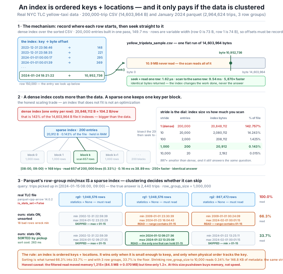
10,952,736, and seek() jumps there in 1.62 µs where a scan reads 10.9 MB it does not want and takes 9.54 ms — 5,870×, identical bytes. Middle — the honest trade: a dense index costs 20,848,112 B against a 14,603,964 B file, 143% of the data it indexes, which is no optimization at all. One entry per 1,000-row block instead costs 20,912 B (997× smaller), and still answers [08:00, 09:00) with the same 168 trips by reading 657 of 200,000 lines (0.33%). Bottom — the same structure, already in the file: parquet's row-group min/max is that sparse index — except CityFlow's real month has is_stats_set = False and carries none, so pushdown reads 100%. Writing statistics ourselves only reaches 66.3%, because 18 dirty timestamps out of 2,964,624 wreck every minimum and the data is 43.53% out of order. Sorting first gives each row group a disjoint slice of time and drops the read to 33.7% — the floor for 3 row groups. An index only helps when the data's physical order tracks the key. Timings vary by machine and run; the ratios and the mechanism are the point.Check the file, not the format’s reputation
The habit this lesson should leave you with is one line long, and it would have settled every assumption above before it was made: read pq.ParquetFile(path).metadata and print md.row_group(0).column(j).statistics.
If that prints None, pushdown cannot skip anything on this file, no matter what the format supports. If it prints a range that spans your whole dataset, the statistics exist but are worthless — check for outliers first, then check whether the data is actually sorted by that column. Only when the ranges come back tight and disjoint does “parquet does predicate pushdown” mean what you hope it means. The footer is a few kilobytes and it answers the question directly — guessing does not.
Exercise 1 — Find the stride that costs one page of memory. The lesson priced strides 1, 10, 100, 1,000 and 10,000 over the 200,000-row CSV, and picked 1,000 somewhat arbitrarily. Make the choice properly: for each stride, measure both the index size in bytes and the average number of lines range_sparse actually reads across ten different one-hour windows spread through the month. Plot or print the two columns side by side and identify the stride where the index first drops under 64 KB. Then explain in a comment which cost you would rather pay, and why the answer depends on how many files CityFlow has to index at once.
Hint
keys and offsets are still in scope, so keys[::stride] rebuilds a sparse index instantly — no need to re-read the file. Rebuild sparse_keys/sparse_off inside your loop, or better, make range_sparse take the index as an argument instead of closing over globals. Generate the ten windows with something like datetime.datetime(2024, 1, d, 8, 0, 0) for d in a spread of days, and format them back to "%Y-%m-%d %H:%M:%S" strings so they compare correctly against the text keys. Expect lines-read to grow roughly linearly with stride while index size shrinks linearly — the product is roughly constant, which is exactly why there is no universally correct stride, only one that fits your memory budget.
Exercise 2 — Prove the 18 outliers are the whole problem. The unsorted file’s statistics were ruined by 18 rows with pickup times outside January 2024. Test that claim directly: filter trips down to rows whose tpep_pickup_datetime falls inside January 2024, write it unsorted with statistics on, and print the row-group min/max. Then run pushdown_report on it and compare the percentage read against the 66.3% the dirty unsorted file managed. Explain in a comment whether cleaning alone was enough, and why.
Hint
Use pc.and_(pc.greater_equal(...), pc.less(...)) to build the mask and trips.filter(mask) to apply it. You will find the minimums become believable January dates — but do not expect the percentage read to reach the sorted file’s 33.7%, because cleaning fixes the outliers and does nothing about the 43.53% of rows that are out of order. The ranges will still overlap heavily, because a row group of a million rows drawn from a loosely-shuffled month still spans most of the month. This is the lesson’s point in miniature: clean data makes bounds correct, sorted data makes bounds tight, and only tight bounds skip.
Exercise 3 — Index a different column and watch it fail. Everything above indexed the column the data was sorted by. Take trips_sorted-style data (sort by pickup time as the lesson does), write it with statistics on, and then run a pushdown report for a filter on PULocationID equal to 132 (JFK Airport, the busiest pickup zone in the month with 145,240 trips) instead of a time window. Report how many row groups survive, and explain in a comment why the min/max index on PULocationID is useless here even though it exists and is perfectly correct.
Hint
Build the filter with ds.field("PULocationID") == 132 and pass it where window was used — you will need a version of pushdown_report that takes the expression as a parameter. Read the PULocationID statistics off each row group with m.row_group(i).column(1).statistics and look at the ranges before you run the report; that will tell you the answer before the measurement does. JFK trips happen at all hours of every day, so sorting by time scatters zone 132 across every row group, and each group’s PULocationID range will be roughly [1, 265]. A table can only be clustered by one key at a time — which is why real databases make you choose a clustering key, and why the next-best tool for the other columns is a secondary index or a bloom filter, not min/max.
You made an index physical. A byte-offset index over the real 200,000-trip CSV recorded that row 150,000 begins at byte 10,952,736, and file.seek() fetched it in 1.62 µs against a scan’s 9.54 ms — 5,870x, identical bytes — because rows are variable width (73 bytes, then 74), so a location that cannot be computed must be recorded. Then the measurement that saves you from the naive version: that dense index weighs 20,848,112 bytes against a 14,603,964-byte file — 143% of the data it indexes — because a 104.2 B/row entry pointing at a ~73-byte row can never pay. Sparse indexing fixed it by having fewer entries, not smaller ones: one key per 1,000-row block costs 20,912 bytes (997x smaller, 0.143% of the file) and answers [08:00, 09:00) with the identical 168 trips by reading 657 of 200,000 lines (0.33%), 250x faster. That structure — ordered keys, one entry per block, bisect then scan locally — is what parquet’s row-group statistics are. Except CityFlow’s real month carries is_stats_set = False: no statistics at all, so pushdown reads 100% of 2,964,624 rows to find 2,440. Writing them ourselves reached only 66.3%, because 18 rows out of 2,964,624 (0.0006%) hold timestamps from 2002 and 2009 that drag every minimum back two decades, and 43.53% of adjacent rows are out of order. Sorting first — 263 ms — gave each row group a disjoint slice of time and dropped the read to 33.7%, the floor for a 3-row-group file; shrinking row_group_size to 10,000 reaches 0.34% for 146.8 KB of footer, the same stride dial in different clothes. And the honest caveat: the filtered read cut memory 1,215x (84.5 MB → 0.070 MB) but time only 1.2x. Pushdown buys memory first.
seek instead of scan, which is why row 150,000 costs 1.62 µs to reach instead of 9.54 ms. It exists because real rows are variable width: 73 bytes then 74, so position cannot be computed by arithmetic and must be recorded at build time. Same bargain as every ordered structure in this module — pay one pass up front, skip forever after.bisect finds the block and a bounded local scan finishes the job. The stride is a dial trading index size against local scan, with no universally right setting; row_group_size is that same dial inside parquet.is_stats_set before planning around pushdown.CityFlow’s dashboard asks for one hour of a month — 2,440 rows out of 2,964,624 — and the file it asks is one you now know three uncomfortable things about: it ships no statistics, 18 of its rows are garbage, and 43.53% of it is out of order. None of that is visible from the outside. A teammate who reads that parquet supports predicate pushdown, writes the filter, and ships it will get correct answers while reading 100% of the file forever, and nothing will ever tell them. The habit that separates you from that outcome is small and mechanical: open the footer and look. Then, if the index isn’t there or isn’t tight, you know exactly which lever to pull, because you have now measured all of them — write the statistics, clean the outliers that widen the bounds, sort by the key you actually filter on, and size the blocks to the granularity your queries need. That is also the module’s spine arriving at its destination. Hashing (Module 6) gave you exact match and threw away order; order is what lets you skip, and skipping is the only thing that makes a question about 2,440 rows cost 2,440 rows’ worth of work. Every database you will ever use is doing what you just did by hand: keeping a small ordered map of keys to locations, and quietly hoping you sorted your data by the thing you’re about to ask about.
Everything in this lesson was a piece measured on its own bench: a byte-offset index on the CSV, a stride dial priced but never tuned against a real workload, statistics read from a file that turned out not to have any, and a sort that we proved was the difference between 66.3% and 33.7% before deleting the file it produced. Lesson 5, the guided project Time-Range Index, is where those pieces become one artifact you would actually ship — a reusable time-range index over the real month, built once and then interrogated for “trips 8-9am” and measured honestly against a full scan. The order of operations there is not an implementation detail, it is this lesson’s conclusion turned into a spec: the project sorts before it indexes, because you have now seen with your own measurement that an index over unclustered data is a correct structure that skips almost nothing. You will also finally spend the crossover method from Module 6 on something that costs real money to build — a sort is , far more expensive than the cheap in-memory pass that made indexing an easy yes back then — so the question “is this index worth building?” gets a genuinely interesting answer for the first time.
Keep DATATWEETS free. Help fund practical data, AI, and engineering lessons for learners worldwide.
