Title here
Summary here
Module 6 ended with a service that could tell you anything about a zone instantly. zone_index[132] returns JFK Airport’s 145,240 trips in constant time, and no amount of extra data slows it down. Then CityFlow’s dashboard team asked for a filter that looks just as innocent: let the user drag a slider and see the trips between 08:00 and 09:00 on January 15th. That question broke the dict, because hashing deliberately scatters neighbouring keys — nothing about 08:00’s slot tells you where 08:01 lives. Over the last four lessons you bought back the property hashing throws away. Lesson 1 unwound problems recursively, Lesson 2 showed that order buys logarithmic search and that bisect over a sorted array is the practical, cache-friendly form of a search tree, Lesson 3 merged sorted runs that don’t fit in memory, and Lesson 4 established the rule this whole project turns on: an index only helps if the data’s physical order correlates with the key.
This project builds the thing those four lessons were for — a reusable time-range index over the real 2,964,624-row January month — and it earns its keep by taking Lesson 4’s rule seriously instead of assuming it. The obvious plan is to index the file as delivered. The first measurement in this lesson kills that plan: the month is not sorted by pickup time, 43.5% of adjacent rows step backwards, and its three row groups each span more than 5,000 days, so a min/max index over the data as shipped can skip nothing whatsoever. So the sort becomes the project, measured honestly and paid for once: 0.93 s to order and cluster the month, producing a 46-entry, 4.3 KB index that answers any 1-hour window with two bisect probes and one bounded read — 2,440 trips between 08:00 and 09:00 on January 15th, in 0.730 ms against a full scan’s 33.01 ms, touching 2.2% of the file, with rows identical to the baseline on every window tested.
By the end of this project, you will be able to:
bisect index into one artifactYou’ll need pyarrow, pandas, numpy, and Python’s standard library (bisect, heapq, resource, multiprocessing).
Before any code, write down what “done” means. A guided project without acceptance criteria is just typing.
CityFlow’s time-range index must, given a month of trip records, answer the question “which trips were picked up in the window ?” — fast, repeatedly, and from a process that never holds the month in memory.
It must satisfy these constraints:
dropna().The data is New York City’s public-domain Yellow Taxi trip records, published by the NYC Taxi & Limousine Commission on its Trip Record Data page — the same January 2024 month you have been streaming since Module 4:
https://d37ci6vzurychx.cloudfront.net/trip-data/yellow_tripdata_2024-01.parquet (2,964,624 rows, 48 MB)https://datatweets.com/datasets/nyc-taxi/taxi_zone_lookup.csv (265 zones)A real pipeline downloads once and then reads the local cached copy, so every runnable block below reads the bare filenames:
# gate: skip
# Fetch once; every block afterwards reads the local cached copies by name.
import urllib.request
urllib.request.urlretrieve(
    "https://d37ci6vzurychx.cloudfront.net/trip-data/yellow_tripdata_2024-01.parquet",
    "yellow_tripdata_2024-01.parquet")
urllib.request.urlretrieve(
    "https://datatweets.com/datasets/nyc-taxi/taxi_zone_lookup.csv",
"taxi_zone_lookup.csv")This is the question the entire design hangs on, and it is the one most tutorials skip. Lesson 4’s rule was blunt: an index over a file only lets you skip parts of that file if the rows are physically arranged so that a key range corresponds to a byte range. If the timestamps are scattered through the file at random, then every block contains trips from every hour, every block overlaps every window, and the world’s best index will still make you read everything.
There is a strong prior that a taxi feed is time-ordered — it is generated by meters, in time order, and the file’s name is the month. That prior is exactly why it needs checking. Note the cheap move that makes the check affordable: we read the key column only. One column of 2.96 million timestamps is 23.7 MB, not the ~400 MB the full month costs in pandas, so the entire investigation runs in a few hundred milliseconds.
import warnings; warnings.filterwarnings("ignore")
import time, bisect, os, sys, heapq, resource, statistics
import datetime as dt
import multiprocessing as mp
import numpy as np
import pyarrow as pa
import pyarrow.parquet as pq
import pyarrow.compute as pc

MONTH = "yellow_tripdata_2024-01.parquet"
CLUSTERED = "l5_clustered.parquet"
QUARANTINE = "l5_quarantine.parquet"
KEY = "tpep_pickup_datetime"
COLS = ["tpep_pickup_datetime", "tpep_dropoff_datetime", "PULocationID",
        "DOLocationID", "trip_distance", "fare_amount", "total_amount"]
DOMAIN_LO = dt.datetime(2024, 1, 1)
DOMAIN_HI = dt.datetime(2024, 2, 1)
BLOCK = 65_536


def pickup_seconds(path=MONTH):
    """The key column alone, as int64 seconds -- 8 bytes a row, not 400 MB."""
    col = pq.read_table(path, columns=[KEY]).column(0)
    return col.to_numpy(zero_copy_only=False).astype("datetime64[s]").view("int64")


def as_dt(x):
    return np.array([x], dtype="int64").view("datetime64[s]")[0]


if __name__ == "__main__":
    ts = pickup_seconds()
    n = len(ts)
    steps = np.diff(ts)
    descents = int((steps < 0).sum())
    print(f"trips in the month     : {n:,}")
    print(f"pickup time min / max  : {as_dt(ts.min())}  ..  {as_dt(ts.max())}")
    print(f"already sorted?        : {bool((steps >= 0).all())}")
    print(f"adjacent pairs that go BACKWARDS: {descents:,} ({descents/len(steps)*100:.1f}%)")
    print(f"median backward jump   : {int(np.median(-steps[steps < 0])):,} s")
    print(f"key column in memory   : {ts.nbytes/1e6:.1f} MB  (the 7-column projection is far bigger)")
trips in the month : 2,964,624
pickup time min / max : 2002-12-31T22:59:39 .. 2024-02-01T00:01:15
already sorted? : False
adjacent pairs that go BACKWARDS: 1,290,558 (43.5%)
median backward jump : 1,444 s
key column in memory : 23.7 MB (the 7-column projection is far bigger)The prior was wrong, and it was wrong in an interesting way. The month is not sorted: 1,290,558 adjacent pairs — 43.5%, very nearly half — step backwards in time. This is not a file with a few records out of place. It is a file where a coin flip decides whether the next row is later than this one.
But look at the median backward jump: 1,444 seconds, about twenty-four minutes. The typical violation is small. This is not random scatter; it is a feed that is roughly time-ordered and locally shuffled, exactly what you would expect from meters reporting independently with their own lag. That distinction matters enormously, and Step 1 is not finished until we know which side of the line it falls on.
The min should also stop you cold. The earliest pickup in the January 2024 file is 2002-12-31T22:59:39 — twenty-one years early.
Before measuring the correlation, deal with the timestamps that are simply wrong, because they turn out to matter far more than their count suggests.
if __name__ == "__main__":
    lo_i = np.datetime64(DOMAIN_LO).astype("datetime64[s]").view("int64")
    hi_i = np.datetime64(DOMAIN_HI).astype("datetime64[s]").view("int64")
    out = (ts < lo_i) | (ts >= hi_i)
    print(f"rows outside [{DOMAIN_LO.date()}, {DOMAIN_HI.date()}): {int(out.sum())} "
          f"({len(set(ts[out].tolist()))} distinct timestamps)")
    print("the offending timestamps:")
    for v in sorted(set(ts[out].tolist())):
        print("   ", as_dt(v))
    inrange = ~out
    corr = np.corrcoef(np.arange(n)[inrange], ts[inrange])[0, 1]
    print(f"corr(row position, pickup time) on the in-range rows: {corr:.4f}")
rows outside [2024-01-01, 2024-02-01): 18 (17 distinct timestamps)
the offending timestamps:
2002-12-31T22:59:39
2009-01-01T00:24:09
2009-01-01T23:30:39
2009-01-01T23:58:40
2023-12-31T23:39:17
2023-12-31T23:41:02
2023-12-31T23:47:28
2023-12-31T23:49:12
2023-12-31T23:54:27
2023-12-31T23:56:45
2023-12-31T23:56:46
2023-12-31T23:57:17
2023-12-31T23:58:35
2023-12-31T23:58:37
2024-02-01T00:00:17
2024-02-01T00:00:39
2024-02-01T00:01:15
corr(row position, pickup time) on the in-range rows: 0.9075Eighteen rows out of 2,964,624 — 0.0006% of the month — fall outside January 2024. They are not one kind of error, either. The ten from 2023-12-31T23:39 to 23:58 are almost certainly real trips that began minutes before midnight and got swept into the January file; the three at 2024-02-01T00:00 are the same thing at the other end. The 2009 and 2002 records are meter or entry faults with no defensible reading.
Now the correlation, computed on the rows that are actually in range: 0.9075. That is the number that explains everything about this file. The month is strongly, but not perfectly, time-ordered. Row position predicts pickup time well — and, as the next step proves, “well” is not the same as “well enough.”
Eighteen rows can cost you the whole index
An index built on min/max per block is only as tight as its extremes, and extremes are exactly what dirty data corrupts. One 2002 record inside a block drags that block’s min back twenty-one years, and from then on the block’s advertised range is “2002 to now” — which overlaps every query you will ever run. The block gets read every single time, forever, because of one row. This is why “18 rows out of 2.96 million, who cares” is the wrong instinct: their count is irrelevant, their position in the sort order is everything. A single outlier at each end of a block is enough to make min/max statistics useless, and you will see it happen in the next step. Decide your key’s valid domain explicitly, and enforce it at build time.
Correlation of 0.9075 sounds encouraging. Time to convert it into the only number that matters: how much of the file would we still have to read?
Parquet’s own answer comes from row-group statistics — Lesson 4’s point that a Parquet file already ships a real index. So the first question is what this file’s three row groups advertise. The second, printed alongside, is what they would advertise if the junk were removed, which separates “the data is scrambled” from “the data is fine but dirty.”
if __name__ == "__main__":
    pf = pq.ParquetFile(MONTH)
    print("does the file carry min/max statistics pyarrow could push down?")
    print("   is_stats_set :", pf.metadata.row_group(0).column(1).is_stats_set)
    print()
    print("what the statistics WOULD say, if they were there:")
    print(f"{'row group':<10} {'rows':>10}  {'min pickup':<20} {'max pickup':<20} {'span':>10}")
    off = 0
    for i in range(pf.metadata.num_row_groups):
        rows = pf.metadata.row_group(i).num_rows
        seg = ts[off:off + rows]
        clean = seg[(seg >= lo_i) & (seg < hi_i)]
        print(f"rg{i:<8} {rows:>10,}  {str(as_dt(seg.min())):<20} {str(as_dt(seg.max())):<20} "
              f"{(seg.max()-seg.min())/86400:>8.0f} d")
        print(f"{'  (junk out)':<10} {len(clean):>10,}  {str(as_dt(clean.min())):<20} "
              f"{str(as_dt(clean.max())):<20} {(clean.max()-clean.min())/86400:>8.1f} d")
        off += rows
does the file carry min/max statistics pyarrow could push down?
is_stats_set : False
what the statistics WOULD say, if they were there:
row group rows min pickup max pickup span
rg0 1,048,576 2002-12-31T22:59:39 2024-01-13T23:51:06 7683 d
(junk out) 1,048,563 2024-01-01T00:00:00 2024-01-13T23:51:06 13.0 d
rg1 1,048,576 2009-01-01T23:30:39 2024-01-24T16:08:30 5501 d
(junk out) 1,048,575 2024-01-13T02:41:01 2024-01-24T16:08:30 11.6 d
rg2 867,472 2009-01-01T00:24:09 2024-02-01T00:01:15 5509 d
(junk out) 867,468 2024-01-01T00:00:58 2024-01-31T23:59:55 31.0 dTwo findings, and they compound.
First: this file carries no statistics at all. is_stats_set is False for every column. The TLC’s writer produced a Parquet file with no min/max metadata, so there is literally nothing for pyarrow to push down. Lesson 4’s built-in index — the one every Parquet file is supposed to ship — is simply absent here. That alone forces us to build our own.
Second, and worse: even if the statistics existed, they would skip almost nothing. Look at the spans. The three row groups advertise 7,683, 5,501 and 5,509 days — every one of them claims to contain trips from 2002 or 2009 through late January, so every one of them overlaps every window you could ask for. Skipping: zero.
And now the crucial part, the line that separates the two diagnoses. Strip the junk and the spans collapse to 13.0, 11.6 and 31.0 days — the data really is roughly ordered, just as the 0.9075 correlation promised. But roughly is not enough. A row group here holds 1,048,576 rows covering about two weeks, so for a 1-hour window on January 15th, rg0 (which ends January 13th) can be skipped while rg1 and rg2 both overlap — two of three row groups, about 67% of the file, to retrieve a few thousand rows. The chunks are simply too coarse to resolve an hour, and rg2 spans the entire month on its own.
There is one more version of the cheap plan worth testing before we commit to sorting. What if we keep the rows exactly where they are and merely re-chunk the file into smaller blocks? Finer granularity, no expensive sort. With 46 blocks of 65,536 rows instead of 3 giant ones, each block covers a much shorter slice of time — and a 0.9075 correlation suggests that might be enough.
if __name__ == "__main__":
    q_lo = dt.datetime(2024, 1, 15, 8, 0)
    q_hi = dt.datetime(2024, 1, 15, 9, 0)
    ql = np.datetime64(q_lo).astype("datetime64[s]").view("int64")
    qh = np.datetime64(q_hi).astype("datetime64[s]").view("int64")

    nb = (n + BLOCK - 1) // BLOCK
    bmin = np.array([ts[i*BLOCK:(i+1)*BLOCK].min() for i in range(nb)])
    bmax = np.array([ts[i*BLOCK:(i+1)*BLOCK].max() for i in range(nb)])
    hit = np.where((bmin < qh) & (bmax >= ql))[0]
    total = int(((ts >= ql) & (ts < qh)).sum())
    print(f"re-chunked to {nb} blocks of {BLOCK:,} rows, still in delivered order")
    print(f"window 2024-01-15 08:00-09:00 truly matches {total:,} rows "
          f"({total/n*100:.3f}% of the month)")
    print(f"blocks a min/max index would make us read: {len(hit)}/{nb} -> {hit.tolist()}")
    for i in hit:
        seg = ts[i*BLOCK:(i+1)*BLOCK]
        got = int(((seg >= ql) & (seg < qh)).sum())
        print(f"   block {i:>2}: {got:>5,} matching rows   (min={as_dt(seg.min())})")
    print(f"blocks whose min is dragged before 2024 by junk: "
          f"{int((bmin < lo_i).sum())} -> read on EVERY query")
re-chunked to 46 blocks of 65,536 rows, still in delivered order
window 2024-01-15 08:00-09:00 truly matches 2,440 rows (0.082% of the month)
blocks a min/max index would make us read: 3/46 -> [18, 39, 43]
block 18: 2,342 matching rows (min=2009-01-01T23:30:39)
block 39: 0 matching rows (min=2009-01-01T00:24:09)
block 43: 98 matching rows (min=2024-01-01T00:00:58)
blocks whose min is dragged before 2024 by junk: 3 -> read on EVERY queryThis is the most instructive output in the lesson, and 3 out of 46 looks like a success until you read the breakdown.
Block 39 contains zero matching rows. We read 65,536 rows off disk to find nothing, and we did it because a single 2009-01-01 record dragged that block’s min back fifteen years. Its advertised range is “2009 to sometime in January,” so it overlaps everything. The callout’s warning, measured: 3 blocks are junk-poisoned, and those 3 get read on every query anyone ever runs. For this particular window they happen to be most of the answer, which is a coincidence, not a design.
And the real rows are split. The window’s 2,440 trips are not in one place: 2,342 sit in block 18 and 98 sit in block 43, thirty-two megabytes away. That is what a 0.9075 correlation looks like from the inside — good enough that most of an hour lands together, not good enough that all of it does. Every query pays for the fragmentation, and there is no bound on how bad it gets: a window that straddles a boundary is worse.
So the cheap plan is dead on evidence, and the verdict is precise rather than vague. The delivered order is nearly useful, and “nearly” costs a wasted 65,536-row read on every query plus a permanently poisoned floor. Order is the property we need, and this file does not have it. We have to buy it.
Now the price. Sorting 2.96 million rows is the expensive step in this whole project, and there are two honest ways to do it, one of which is the technique Lesson 3 built.
The in-memory sort reads the 7-column projection, filters it to the domain, and hands the whole thing to pyarrow’s sort_by — a single C-level sort over an Arrow table.
The external sort is Lesson 3’s answer for data that doesn’t fit: sort each row group into a sorted run on disk, then merge the runs with heapq.merge, which pulls from three sorted streams and yields one sorted stream while holding only one row from each in memory. It is the technique that still works when the input is a year, not a month.
Both implement the same junk policy, and it is worth stating plainly: out-of-domain rows are quarantined, not deleted. They go to their own file, where a data engineer can look at them, rather than vanishing into a dropna() that no one ever hears about again.
def sort_in_memory(src=MONTH, out=CLUSTERED, quarantine=QUARANTINE):
    """Sort the whole projection at once. Fast, but peaks at the projection's size."""
    t = pq.read_table(src, columns=COLS)
    k = t.column(KEY).to_numpy(zero_copy_only=False).astype("datetime64[s]")
    keep = (k >= np.datetime64(DOMAIN_LO)) & (k < np.datetime64(DOMAIN_HI))
    pq.write_table(t.filter(pa.array(~keep)), quarantine)
    t = t.filter(pa.array(keep)).sort_by([(KEY, "ascending")])
    pq.write_table(t, out, row_group_size=BLOCK)
    return t.num_rows, int((~keep).sum())


def sort_external(src=MONTH, out=CLUSTERED, quarantine=QUARANTINE):
    """Lesson 3's external sort: sort each row group into a run, then k-way merge."""
    pfile = pq.ParquetFile(src)
    runs, junk = [], []
    for i in range(pfile.metadata.num_row_groups):
        t = pfile.read_row_group(i, columns=COLS)
        k = t.column(KEY).to_numpy(zero_copy_only=False).astype("datetime64[s]")
        keep = (k >= np.datetime64(DOMAIN_LO)) & (k < np.datetime64(DOMAIN_HI))
        junk.append(t.filter(pa.array(~keep)))
        t = t.filter(pa.array(keep)).sort_by([(KEY, "ascending")])
        p = f"l5_run_{i}.parquet"
        pq.write_table(t, p)
        runs.append(p)
        del t
    pq.write_table(pa.concat_tables(junk), quarantine)
    schema = pq.ParquetFile(runs[0]).schema_arrow

    def stream(path):
        f = pq.ParquetFile(path)
        for b in f.iter_batches(batch_size=BLOCK):
            cols = [b.column(c).to_pylist() for c in COLS]
            for row in zip(*cols):
                yield row

    writer, buf, total = None, [], 0

    def flush(writer, buf):
        tb = pa.Table.from_arrays(
            [pa.array([r[j] for r in buf], type=schema.field(j).type)
             for j in range(len(COLS))], names=COLS)
        if writer is None:
            writer = pq.ParquetWriter(out, tb.schema)
        writer.write_table(tb, row_group_size=BLOCK)
        return writer

    for row in heapq.merge(*(stream(p) for p in runs), key=lambda r: r[0]):
        buf.append(row)
        if len(buf) == BLOCK:
            writer = flush(writer, buf); total += len(buf); buf = []
    if buf:
        writer = flush(writer, buf); total += len(buf)
    writer.close()
    for p in runs:
        os.remove(p)
    return total, sum(j.num_rows for j in junk)


if __name__ == "__main__":
    t0 = time.perf_counter()
    kept, junked = sort_in_memory(out="l5_sorted_mem.parquet", quarantine=QUARANTINE)
    t_mem = time.perf_counter() - t0
    print(f"in-memory sort : {t_mem:>6.2f} s  kept {kept:,}  quarantined {junked}")

    t0 = time.perf_counter()
    kept_x, junked_x = sort_external(out="l5_sorted_ext.parquet", quarantine="l5_junk_ext.parquet")
    t_ext = time.perf_counter() - t0
    print(f"external sort  : {t_ext:>6.2f} s  kept {kept_x:,}  quarantined {junked_x}")

    same = pq.read_table("l5_sorted_mem.parquet").equals(pq.read_table("l5_sorted_ext.parquet"))
    print(f"byte-identical output? : {same}")
    print(f"external sort is {t_ext/t_mem:.1f}x SLOWER on this month")

    os.replace("l5_sorted_mem.parquet", CLUSTERED)          # keep the one we chose
    os.remove("l5_sorted_ext.parquet"); os.remove("l5_junk_ext.parquet")
    print(f"clustered file : {os.path.getsize(CLUSTERED)/1e6:.1f} MB, "
          f"{pq.ParquetFile(CLUSTERED).metadata.num_row_groups} row groups")
in-memory sort : 0.93 s kept 2,964,606 quarantined 18
external sort : 13.97 s kept 2,964,606 quarantined 18
byte-identical output? : True
external sort is 15.0x SLOWER on this month
clustered file : 51.2 MB, 46 row groupsThe two sorts produce byte-identical output — the same 2,964,606 rows in the same order, with the same 18 quarantined — which is the correctness check that lets us choose between them purely on cost. And the cost is not close: the external sort is 15.0x slower, 13.97 s against 0.93 s.
That result deserves to be stated rather than buried, because it contradicts the reflex this module might otherwise install. The external sort is the more sophisticated algorithm, it is the one Lesson 3 taught, and on this data it is fifteen times worse. The reason is not that k-way merging is bad; it is that heapq.merge pulls 2.96 million Python tuples through the interpreter one at a time, while sort_by sorts an Arrow buffer in C without ever creating a Python object. The Python-level merge loses by roughly the margin you would expect any per-row Python loop to lose to vectorized C.
So we use the in-memory sort, and the module keeps the external one for the case it was designed for. That case is real, and Step 8’s measurement will show exactly what it buys: the choice is not “which is faster” but “does the projection fit.”
The sorted file is written in blocks of 65,536 rows, and because we wrote it with pyarrow, it now carries the min/max statistics the original never had. Look at what ordering did to them:
if __name__ == "__main__":
    cf = pq.ParquetFile(CLUSTERED)
    print(f"{'block':<7} {'rows':>8}  {'min pickup':<20} {'max pickup':<20}")
    for i in list(range(3)) + [cf.metadata.num_row_groups - 1]:
        st = cf.metadata.row_group(i).column(0).statistics
        print(f"rg{i:<5} {cf.metadata.row_group(i).num_rows:>8,}  "
              f"{str(st.min):<20} {str(st.max):<20}")
    print("...")
    spans = []
    for i in range(cf.metadata.num_row_groups):
        st = cf.metadata.row_group(i).column(0).statistics
        spans.append((st.max - st.min).total_seconds() / 3600)
    print(f"block time span: median {statistics.median(spans):.1f} h, max {max(spans):.1f} h")
block rows min pickup max pickup
rg0 65,536 2024-01-01 00:00:00 2024-01-01 18:06:24
rg1 65,536 2024-01-01 18:06:25 2024-01-02 17:15:52
rg2 65,536 2024-01-02 17:15:52 2024-01-03 14:56:52
rg45 15,486 2024-01-31 20:56:26 2024-01-31 23:59:55
...
block time span: median 17.7 h, max 23.2 hCompare that to Step 3’s 5,501-to-7,683-day spans. Each block now covers a median of 17.7 hours and at most 23.2 hours, and the blocks tile the month end to end: rg0 stops at 18:06:24 and rg1 starts at 18:06:25. Nothing overlaps, so a window can only live in the one or two blocks that bracket it. This is what clustering means — the physical order now is the key order — and it is the entire reason the next step works.
The index itself is almost embarrassingly small. It is a sorted array of one key per block: the block’s minimum, plus the row number it starts at. That is Lesson 4’s sparse index — and because the array is sorted, Lesson 2’s bisect searches it in without building a single tree node.
def load_index(path=CLUSTERED):
    """The sparse index: one (min key, first row) pair per block. Lesson 4's shape."""
    f = pq.ParquetFile(path)
    keys, starts, row = [], [], 0
    for i in range(f.metadata.num_row_groups):
        keys.append(f.metadata.row_group(i).column(0).statistics.min)
        starts.append(row)
        row += f.metadata.row_group(i).num_rows
    return f, keys, starts


if __name__ == "__main__":
    CF, BLOCK_MIN, BLOCK_START = load_index()
    idx_bytes = (sys.getsizeof(BLOCK_MIN) + sum(sys.getsizeof(x) for x in BLOCK_MIN)
                 + sys.getsizeof(BLOCK_START) + sum(sys.getsizeof(x) for x in BLOCK_START))
    print(f"index entries        : {len(BLOCK_MIN)}")
    print(f"index size in memory : {idx_bytes/1024:.1f} KB")
    print(f"rows it stands in for: {sum(CF.metadata.row_group(i).num_rows for i in range(len(BLOCK_MIN))):,}")
    print(f"bytes of data per index entry: "
          f"{os.path.getsize(CLUSTERED)/len(BLOCK_MIN)/1e6:.2f} MB")
    print(f"first three block mins: {BLOCK_MIN[:3]}")
index entries : 46
index size in memory : 4.3 KB
rows it stands in for: 2,964,606
bytes of data per index entry: 1.11 MB
first three block mins: [datetime.datetime(2024, 1, 1, 0, 0), datetime.datetime(2024, 1, 1, 18, 6, 25), datetime.datetime(2024, 1, 2, 17, 15, 52)]Forty-six entries. 4.3 kilobytes. That is the whole index for 2,964,606 trips — each entry standing in for 1.11 MB of data it lets you skip. This is what “sparse” means and why it is the right choice: a dense index with one entry per row would hold 2.96 million entries to buy you nothing, because you cannot read half a block off a disk anyway. The index’s granularity should match the physical read unit, and here that unit is the block.
Everything now assembles into the query. The two bisect calls are the payoff of the whole module, and the asymmetry between them is worth reading closely.
For the lower bound we need the block that might already contain lo. bisect_right(keys, lo) returns the first block starting strictly after lo, so we step back one: the window’s earliest row lives in the block before that, whose minimum is at or below lo. For the upper bound, bisect_left(keys, hi) is exactly the first block whose minimum is at or beyond hi — that block cannot contain anything below hi, so it becomes the exclusive end. The result is a half-open bracket range(first, last).
Then the only linear work in the entire query: read those blocks and filter the edges, because the first and last block of the bracket generally contain rows on the wrong side of the boundary. That filter is over 65,536 rows, not 2.96 million.
def blocks_for(lo, hi, keys=None):
    """Two O(log n) probes -> the half-open bracket of blocks that can hold [lo, hi)."""
    keys = BLOCK_MIN if keys is None else keys
    first = max(bisect.bisect_right(keys, lo) - 1, 0)
    last = bisect.bisect_left(keys, hi)
    return list(range(first, last))


def query_index(lo, hi):
    """Bisect for the bracket, read only those blocks, filter the edges."""
    groups = blocks_for(lo, hi)
    t = CF.read_row_groups(groups, columns=COLS)
    m = pc.and_(pc.greater_equal(t.column(KEY), pa.scalar(lo)),
                pc.less(t.column(KEY), pa.scalar(hi)))
    return t.filter(m), groups


def query_scan(lo, hi):
    """BASELINE: read the month, filter it, throw the rest away."""
    t = pq.read_table(MONTH, columns=COLS)
    m = pc.and_(pc.greater_equal(t.column(KEY), pa.scalar(lo)),
                pc.less(t.column(KEY), pa.scalar(hi)))
    return t.filter(m)


if __name__ == "__main__":
    res, groups = query_index(q_lo, q_hi)
    print(f"window          : {q_lo} .. {q_hi}")
    print(f"bisect bracket  : blocks {groups} of {len(BLOCK_MIN)}")
    print(f"rows read       : {sum(CF.metadata.row_group(g).num_rows for g in groups):,} "
          f"of {CF.metadata.num_rows:,} "
          f"({sum(CF.metadata.row_group(g).num_rows for g in groups)/CF.metadata.num_rows*100:.1f}%)")
    print(f"rows returned   : {res.num_rows:,}")
window : 2024-01-15 08:00:00 .. 2024-01-15 09:00:00
bisect bracket : blocks [19] of 46
rows read : 65,536 of 2,964,606 (2.2%)
rows returned : 2,440One block out of forty-six. Two integer comparisons’ worth of bisect work over a 46-element array told us that every trip picked up between 08:00 and 09:00 on January 15th is inside block 19 and nowhere else, so we read 65,536 rows — 2.2% of the file — and filtered them down to 2,440. Compare that with Step 4’s delivered order: three blocks, one of them empty, the answer split across two. Sorting turned “3 blocks and a coin flip” into “1 block, guaranteed.”
A fast wrong answer is worthless, and acceptance criterion 3 exists to make that non-negotiable. Before a single timing, the index must return exactly what the dumb full scan returns — not the same count, the same rows. The windows below are chosen to include the awkward cases: a quiet 03:00 hour, and the last hour of the month, which runs up against the domain boundary.
if __name__ == "__main__":
    WINDOWS = [(dt.datetime(2024, 1, d, 8), dt.datetime(2024, 1, d, 9)) for d in (5, 15, 22, 29)]
    WINDOWS += [(dt.datetime(2024, 1, 15, 3), dt.datetime(2024, 1, 15, 4)),
                (dt.datetime(2024, 1, 31, 23), dt.datetime(2024, 2, 1, 0))]
    print(f"{'window':<28} {'index':>7} {'scan':>7} {'blocks':>8} {'identical':>10}")
    all_same = True
    for lo, hi in WINDOWS:
        a, g = query_index(lo, hi)
        b = query_scan(lo, hi)
        same = a.sort_by([(KEY, "ascending")]).equals(b.sort_by([(KEY, "ascending")]))
        all_same &= same
        label = f"{lo:%b %d %H:%M}-{hi:%H:%M}"
        print(f"{label:<28} {a.num_rows:>7,} {b.num_rows:>7,} "
              f"{len(g):>3}/{len(BLOCK_MIN):<4} {str(same):>10}")
    print(f"\nevery window identical to the full scan: {all_same}")
window index scan blocks identical
Jan 05 08:00-09:00 4,225 4,225 1/46 True
Jan 15 08:00-09:00 2,440 2,440 1/46 True
Jan 22 08:00-09:00 4,834 4,834 1/46 True
Jan 29 08:00-09:00 4,417 4,417 2/46 True
Jan 15 03:00-04:00 443 443 1/46 True
Jan 31 23:00-00:00 3,061 3,061 1/46 True
every window identical to the full scan: TrueCriterion 3 is met: identical rows on every window, including the 03:00 lull (443 trips) and the month’s final hour (3,061). Note January 29th needing 2 blocks — its window straddles a block boundary, which is the normal worst case for a sparse index and costs exactly one extra block, not a re-scan. That bound is the point: 1 or 2 blocks, always, never 46.
Now the timings. Each window is warmed first, then the index is timed over 20 runs and the scan over 5, and medians are reported — a single perf_counter reading on a sub-millisecond operation is noise, not data.
if __name__ == "__main__":
    idx_ms, scan_ms = [], []
    for lo, hi in WINDOWS[:4]:
        query_index(lo, hi); query_scan(lo, hi)          # warm the cache
        a = []
        for _ in range(20):
            t0 = time.perf_counter(); query_index(lo, hi); a.append((time.perf_counter()-t0)*1000)
        b = []
        for _ in range(5):
            t0 = time.perf_counter(); query_scan(lo, hi); b.append((time.perf_counter()-t0)*1000)
        idx_ms.append(statistics.median(a)); scan_ms.append(statistics.median(b))
        print(f"{lo:%b %d %H:%M}  index {statistics.median(a):>7.3f} ms   "
              f"scan {statistics.median(b):>7.2f} ms   {statistics.median(b)/statistics.median(a):>5.1f}x")
    IDX = statistics.median(idx_ms); SCAN = statistics.median(scan_ms)
    print(f"\nmedian index query : {IDX:.3f} ms")
    print(f"median full scan   : {SCAN:.2f} ms")
    print(f"speedup            : {SCAN/IDX:.1f}x")
    CROSS = (t_mem * 1000) / (SCAN - IDX)
    print(f"\nbuild cost {t_mem*1000:.0f} ms / saving {SCAN-IDX:.2f} ms per query "
          f"-> pays for itself after {CROSS:.1f} queries")
Jan 05 08:00 index 0.766 ms scan 32.82 ms 42.8x
Jan 15 08:00 index 0.694 ms scan 32.93 ms 47.5x
Jan 22 08:00 index 0.681 ms scan 33.39 ms 49.1x
Jan 29 08:00 index 1.274 ms scan 33.08 ms 26.0x
median index query : 0.730 ms
median full scan : 33.01 ms
speedup : 45.2x
build cost 934 ms / saving 32.28 ms per query -> pays for itself after 28.9 queries45.2x, and the structure of the table matters more than the headline. The three single-block windows land at 0.68–0.77 ms; January 29th, the two-block case, costs 1.274 ms — almost exactly double, and still 26x faster than the scan. That linearity is the index behaving exactly as designed: cost tracks blocks read, and blocks read is bounded by the window, never by the file.
The crossover is 28.9 queries. Building the index costs 934 ms and each query saves 32.28 ms, so the twenty-ninth query is where the sort has paid for itself and everything after is profit. Be honest about what that number means: this is a far worse crossover than Module 6’s index-versus-scan 4.4 queries, and the reason is that the baseline here is good. pq.read_table on a 48 MB file with a 7-column projection is a vectorized, multi-threaded, page-cached C read — 33 ms is genuinely quick. The index is not beating a strawman. For a dashboard that answers thousands of window queries a day, 28.9 is paid back before the first coffee; for a script that asks one question and exits, the index is a waste of time and you should just scan. That is the honest engineering call, and it depends entirely on the query volume.
Time is only half of it, and for this course it has never been the important half. Memory needs its own harness, for a reason worth repeating: tracemalloc distorts the timings badly, so it must never share a block with a stopwatch. We use resource.getrusage(RUSAGE_SELF).ru_maxrss, the operating system’s high-water mark of resident memory, which counts everything tracemalloc cannot see — the interpreter, the pandas and pyarrow C extensions, and the large Arrow buffers underneath a table.
ru_maxrss never falls, so each variant gets a fresh spawned interpreter and reports its own peak, exactly as Module 6’s project did. The imports only row establishes the floor that belongs to neither implementation.
def peak_mb():
    kb = resource.getrusage(resource.RUSAGE_SELF).ru_maxrss
    return kb / (1024*1024) if sys.platform == "darwin" else kb / 1024


def _m_floor(q):
    q.put(("imports only", 0.0, peak_mb()))


def _m_pandas(q):
    import pandas as pd
    t0 = time.perf_counter()
    df = pd.read_parquet(MONTH)
    w = df[(df[KEY] >= dt.datetime(2024, 1, 15, 8)) & (df[KEY] < dt.datetime(2024, 1, 15, 9))]
    q.put(("pandas scan (all cols)", time.perf_counter()-t0, peak_mb()))


def _m_scan(q):
    t0 = time.perf_counter()
    r = query_scan(dt.datetime(2024, 1, 15, 8), dt.datetime(2024, 1, 15, 9))
    q.put(("arrow scan (7 cols)", time.perf_counter()-t0, peak_mb()))


def _m_index(q):
    global CF, BLOCK_MIN, BLOCK_START
    CF, BLOCK_MIN, BLOCK_START = load_index()
    t0 = time.perf_counter()
    r, g = query_index(dt.datetime(2024, 1, 15, 8), dt.datetime(2024, 1, 15, 9))
    q.put(("index query", time.perf_counter()-t0, peak_mb()))


if __name__ == "__main__":
    ctx = mp.get_context("spawn")
    mrows = []
    for fn in (_m_floor, _m_pandas, _m_scan, _m_index):
        qq = ctx.Queue(); pr = ctx.Process(target=fn, args=(qq,))
        pr.start(); mrows.append(qq.get()); pr.join()
    print(f"{'variant':<24} {'time':>8} {'peak RSS':>10} {'over floor':>11}")
    floor = mrows[0][2]
    for w, s, m in mrows:
        print(f"{w:<24} {s:>7.2f}s {m:>7.0f} MB {m-floor:>8.0f} MB")
variant time peak RSS over floor
imports only 0.00s 61 MB 0 MB
pandas scan (all cols) 0.28s 1008 MB 947 MB
arrow scan (7 cols) 0.32s 317 MB 256 MB
index query 0.26s 109 MB 48 MBHere is the result the acceptance criteria were really about. The dashboard’s naive move — pd.read_parquet then filter — peaks at 1,008 MB, which is the “~400 MB into pandas” of the brief plus Arrow’s read buffers on the way in. The disciplined Arrow scan with a 7-column projection is much better at 317 MB. And the index query peaks at 109 MB — just 48 MB above the bare-interpreter floor, because it never holds more than one 65,536-row block.
That is a 9.2x reduction against the pandas baseline, and unlike the crossover it is collected on the very first query. More importantly it is the number that doesn’t move when the data grows: feed this a year of trips and the pandas baseline needs twelve times the RAM, while the index still reads one block per window and still peaks around 109 MB. The index’s memory is bounded by the block size, not the file size.
Now the build side, which is where the external sort finally gets to make its case:
def _m_sort_mem(q):
    t0 = time.perf_counter(); sort_in_memory(out="l5_tmp_mem.parquet", quarantine="l5_tmp_qm.parquet")
    q.put(("in-memory sort", time.perf_counter()-t0, peak_mb()))


def _m_sort_ext(q):
    t0 = time.perf_counter(); sort_external(out="l5_tmp_ext.parquet", quarantine="l5_tmp_qx.parquet")
    q.put(("external sort", time.perf_counter()-t0, peak_mb()))


if __name__ == "__main__":
    brows = []
    for fn in (_m_floor, _m_sort_mem, _m_sort_ext):
        qq = ctx.Queue(); pr = ctx.Process(target=fn, args=(qq,))
        pr.start(); brows.append(qq.get()); pr.join()
    print(f"{'build strategy':<24} {'time':>8} {'peak RSS':>10}")
    for w, s, m in brows:
        print(f"{w:<24} {s:>7.2f}s {m:>7.0f} MB")
    print(f"\nexternal sort: {brows[2][1]/brows[1][1]:.1f}x the time, "
          f"{brows[1][2]-brows[2][2]:.0f} MB less peak")
    for f in ("l5_tmp_mem.parquet", "l5_tmp_ext.parquet", "l5_tmp_qm.parquet", "l5_tmp_qx.parquet"):
        if os.path.exists(f):
            os.remove(f)
build strategy time peak RSS
imports only 0.00s 60 MB
in-memory sort 1.35s 628 MB
external sort 14.25s 426 MB
external sort: 10.6x the time, 202 MB less peakAnd there is the trade, stated in two numbers: the external sort costs 10.6x the time to save 202 MB of peak. On a 48 MB month that is a bad deal and we correctly rejected it. But read the shape rather than the values. The in-memory sort’s 628 MB is a function of the input size — it holds the entire projection at once, so a year of trips would ask for roughly 7 GB and the process would die. The external sort’s 426 MB is a function of the run size, which you choose. It is slower on purpose, and what it buys is not speed but the ability to finish at all.
This is precisely the lesson Module 6 learned when its bounded heap turned out slower than nlargest: the sophisticated structure was buying memory, not time. Same shape, one module later, at file scale. Pick the in-memory sort while the projection fits; switch to the external one at the size where “fits” stops being true — and know that number in advance rather than discovering it at 3 a.m.
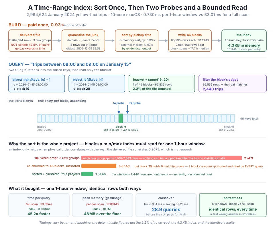
min. Sorting and clustering once for 0.93 s collapses the block spans to a 17.7 h median and yields a 46-entry, 4.3 KB index: two bisect probes bracket the window to 1 of 46 blocks, and reading 2.2% of the file returns 2,440 trips in 0.730 ms against the full scan's 33.01 ms, at 109 MB peak instead of the pandas baseline's 1,008 MB. Measured on a 10-core macOS machine with getrusage, each variant in its own spawned process; timings vary by run, the 2.2% and the identical results do not.Acceptance criterion 4 said every structure earns its place, and that only means something if you are willing to reject some. Four candidates were considered and rejected, and the reasons are the module in miniature.
A dict keyed by timestamp. This is where Module 7 started and it is worth restating, because it is the reason the module exists. A hash index would answer trips_at["2024-01-15 08:00:00"] instantly and would be completely useless here, because hashing scatters neighbouring keys on purpose. There is no way to ask a dict for “everything between two keys” short of visiting all of them. Range queries need order; hashing destroys order. That is not a flaw in dicts, it is their design.
A real binary search tree. Lesson 2 made this case and the index above is the proof. A node-based BST over 46 keys would mean 46 objects, 92 pointers, and a cache miss at every hop, to reproduce exactly what bisect does on a flat sorted array with no allocation at all. The sorted array is the tree, flattened — same , better constants, one-tenth the code. Node-based trees earn their place when the structure must be modified cheaply, which brings us to the honest caveat: our index is immutable, and rebuilding it means re-sorting. A database uses a B-tree precisely because it must support inserts. CityFlow’s month is a static file, so we don’t pay for what we don’t use.
A dense index, one entry per row. 2,964,606 entries instead of 46, to buy nothing, because you cannot read half a block off a disk. The index’s granularity should match the physical read unit. Sparse is not a compromise here; it is the correct answer.
Parquet’s own predicate pushdown. This one deserves a measurement rather than an assertion, because it is the strongest alternative and it very nearly wins:
if __name__ == "__main__":
    def pushdown(path):
        return pq.read_table(path, columns=COLS,
                             filters=[(KEY, ">=", q_lo), (KEY, "<", q_hi)])
    for path, label in ((MONTH, "pushdown, delivered order"), (CLUSTERED, "pushdown, clustered")):
        r = pushdown(path)
        tt = []
        for _ in range(10):
            t0 = time.perf_counter(); pushdown(path); tt.append((time.perf_counter()-t0)*1000)
        print(f"{label:<28} {r.num_rows:>6,} rows  {statistics.median(tt):>7.2f} ms")
    print(f"{'our sparse index':<28} {res.num_rows:>6,} rows  {IDX:>7.2f} ms")
pushdown, delivered order 2,440 rows 32.33 ms
pushdown, clustered 2,440 rows 2.40 ms
our sparse index 2,440 rows 0.73 msThis is the most honest table in the lesson, and it reorders the credit. Pushdown on the delivered file takes 32.33 ms — no better than a full scan, exactly as Step 3 predicted: no statistics to read, and row groups that overlap everything even if there were. Pushdown on the clustered file takes 2.40 ms. Same library call, same query, 13.5x faster, and the only thing that changed was that we sorted the data.
So the headline is not “we hand-built a clever index.” It is: the sort was the win, and pyarrow will happily exploit it for free. Our index adds a further 3.3x on top (2.40 ms to 0.73 ms) by keeping 46 keys resident in a Python list instead of re-opening and re-parsing the file’s metadata on every call — a real gain, but a modest one next to the 13.5x that ordering delivered. If CityFlow only needed this for Parquet, filters= on a sorted file would be a defensible answer and 50 lines lighter.
We keep the explicit index for two reasons that survive that admission. It works on formats that have no statistics — a sorted CSV, a JSONL export, a raw binary file — where filters= has nothing to push down and byte offsets are all you have. And it is inspectable: explain() below tells you how many blocks a query will touch before you run it, which is the difference between a pipeline you can reason about and one you can only benchmark.
Criterion 5: the deliverable is an importable class. Everything above becomes TimeRangeIndex — the artifact you keep and carry into Module 8.
The design separates the two phases that were tangled together in the prototype. build() is the one-time, expensive path: order the data, enforce the domain, quarantine the junk, write the clustered blocks. __init__ is the cheap path: open an already-clustered file and read its 46 keys, which is what a query process does at startup. Everything else is a query method. The strategy argument is the honest result of Step 5 and Step 9 made selectable rather than hard-coded — "memory" while the projection fits, "external" when it does not.
class TimeRangeIndex:
    """CityFlow's time-range index: sorted blocks + bisect + a bounded read."""

    def __init__(self, path, key=KEY, columns=COLS):
        self.path, self.key, self.columns = path, key, columns
        self.file = pq.ParquetFile(path)
        md = self.file.metadata
        self.block_min, self.block_start, row = [], [], 0
        for i in range(md.num_row_groups):
            st = md.row_group(i).column(md.schema.names.index(key)).statistics
            if st is None:
                raise ValueError("clustered file has no statistics -- rebuild it")
            self.block_min.append(st.min)
            self.block_start.append(row)
            row += md.row_group(i).num_rows
        self.rows = row

    @classmethod
    def build(cls, src, out, key=KEY, columns=COLS, domain=(DOMAIN_LO, DOMAIN_HI),
              quarantine=None, block=BLOCK, strategy="memory"):
        """Order the data by `key`, quarantine anything outside `domain`, write blocks."""
        lo, hi = domain
        if strategy == "memory":
            t = pq.read_table(src, columns=columns)
            k = t.column(key).to_numpy(zero_copy_only=False).astype("datetime64[s]")
            keep = (k >= np.datetime64(lo)) & (k < np.datetime64(hi))
            if quarantine:
                pq.write_table(t.filter(pa.array(~keep)), quarantine)
            t = t.filter(pa.array(keep)).sort_by([(key, "ascending")])
            pq.write_table(t, out, row_group_size=block)
        elif strategy == "external":
            sort_external(src=src, out=out, quarantine=quarantine or "l5_junk.parquet")
        else:
            raise ValueError("strategy must be 'memory' or 'external'")
        return cls(out, key=key, columns=columns)

    def blocks_for(self, lo, hi):
        first = max(bisect.bisect_right(self.block_min, lo) - 1, 0)
        return list(range(first, bisect.bisect_left(self.block_min, hi)))

    def query(self, lo, hi, columns=None):
        groups = self.blocks_for(lo, hi)
        if not groups:
            return self.file.read_row_groups([], columns=columns or self.columns)
        t = self.file.read_row_groups(groups, columns=columns or self.columns)
        m = pc.and_(pc.greater_equal(t.column(self.key), pa.scalar(lo)),
                    pc.less(t.column(self.key), pa.scalar(hi)))
        return t.filter(m)

    def count(self, lo, hi):
        return self.query(lo, hi, columns=[self.key]).num_rows

    def explain(self, lo, hi):
        g = self.blocks_for(lo, hi)
        scanned = sum(self.file.metadata.row_group(i).num_rows for i in g)
        return dict(blocks=len(g), of=len(self.block_min), rows_scanned=scanned,
                    pct_of_file=round(scanned / self.rows * 100, 2))


if __name__ == "__main__":
    idx = TimeRangeIndex(CLUSTERED)
    print("plan :", idx.explain(q_lo, q_hi))
    trips = idx.query(q_lo, q_hi)
    print(f"trips between {q_lo:%H:%M} and {q_hi:%H:%M} on {q_lo:%b %d}: {trips.num_rows:,}")
    print(f"count() shortcut : {idx.count(q_lo, q_hi):,}")
    df = trips.to_pandas()
    print(f"average fare     : ${df.fare_amount.mean():.2f}")
    print(f"average distance : {df.trip_distance.mean():.2f} miles")
    print(f"total billed     : ${df.total_amount.sum():,.2f}")
    import pandas as pd
    zones = pd.read_csv("taxi_zone_lookup.csv").set_index("LocationID")["Zone"]
    print("busiest pickup zones in that hour:")
    for zid, c in df.PULocationID.value_counts().head(5).items():
        print(f"   {zones.get(zid, '?'):<32} {c:>4}")
plan : {'blocks': 1, 'of': 46, 'rows_scanned': 65536, 'pct_of_file': 2.21}
trips between 08:00 and 09:00 on Jan 15: 2,440
count() shortcut : 2,440
average fare : $17.53
average distance : 3.36 miles
total billed : $62,725.73
busiest pickup zones in that hour:
Times Sq/Theatre District 207
Penn Station/Madison Sq West 140
Upper East Side North 118
JFK Airport 111
Clinton East 99There is the dashboard’s answer, and it is a real one about a real morning. Between 08:00 and 09:00 on Monday 15 January 2024, New York’s yellow cabs picked up 2,440 fares, averaging $17.53 over 3.36 miles, billing $62,725.73 in that single hour. The rush-hour signature is unmistakable and completely different from the month-wide ranking Module 6 produced: that one was topped by JFK Airport with 145,240 trips, but in the 8 a.m. commuter hour JFK drops to fourth (111) behind Times Square/Theatre District (207), Penn Station/Madison Sq West (140) and Upper East Side North (118). Penn Station at 8 a.m. is commuters off New Jersey Transit; JFK at 8 a.m. is nobody’s flight. The month’s answer and the hour’s answer are different answers — which is the entire reason the dashboard needs a time filter, and the reason this index exists.
Note explain() doing its job: it reported 1 block, 65,536 rows, 2.21% of the file before the query ran. A query planner you can interrogate is worth more than one that is merely fast.
Finally, the quarantine file — the 18 rows we refused to silently drop — and cleanup of everything this lesson wrote:
if __name__ == "__main__":
    junk = pq.read_table(QUARANTINE)
    print(f"quarantined rows: {junk.num_rows}")
    print(junk.column(KEY).to_pandas().sort_values().head(4).to_string(index=False))
    for f in (CLUSTERED, QUARANTINE):
        if os.path.exists(f):
            os.remove(f)
    print("\nwork dir cleaned:", [f for f in os.listdir(".") if f.startswith("l5_")] or "no l5_ files left")
quarantined rows: 18
2002-12-31 22:59:39
2002-12-31 22:59:39
2009-01-01 00:24:09
2009-01-01 23:30:39
work dir cleaned: no l5_ files leftEighteen rows, preserved and inspectable rather than deleted — and note the 2002 timestamp appearing twice, which is why the count is 18 against 17 distinct values. Somewhere in the TLC’s pipeline, two different trips got stamped with the same impossible instant. That is a finding for the data provider, and it exists only because the index quarantined its junk instead of dropping it.
These extend the project. Keep TimeRangeIndex, sort_external, and the local Parquet file exactly as they are.
Exercise 1 — Find the block size that minimises total query cost. The 65,536-row block was inherited from Module 4’s batch size, not chosen. Rebuild the clustered file with block in (4_096, 16_384, 65_536, 262_144) and, for each, report the index’s entry count, its size in KB, and the median time for a 1-hour window. Predict the shape of the curve before running it, then explain the two forces that fight each other.
Hint
Two costs move in opposite directions as blocks shrink. Rows read falls — a 4,096-row block wastes far less on a 2,440-row answer than a 65,536-row block does — but the index grows (724 entries instead of 46) and Parquet’s per-row-group overhead rises, since every block carries its own metadata, its own column chunks, and its own compression dictionaries. Expect the file itself to get bigger and the write to get slower as blocks shrink. Watch for the point where the block is smaller than the answer, at which case you start paying overhead for nothing. Use explain() to report rows_scanned at each size — that is the deterministic number, and it will fall much more cleanly than the noisy millisecond timings.
Exercise 2 — Add a second key and discover why databases only cluster once. The routing team wants query_zone_window(zone, lo, hi) — trips from one pickup zone within a time window. Add it to TimeRangeIndex using the existing time index plus a filter on PULocationID, then measure it for JFK (zone 132) over a 1-hour window against the same query on a file clustered by (PULocationID, tpep_pickup_datetime) instead. Report which wins, and explain what the loser gave up.
Hint
A file has exactly one physical order, so a second sort key is only free within the first. Clustering by (PULocationID, pickup) makes zone-then-time queries read one small bracket, but it destroys the time index: trips from 08:00 are now scattered across all 260-odd zone regions, so a plain time-window query goes back to reading the whole file — you have re-created Step 4’s problem deliberately. This is exactly why a database lets you build many indexes but cluster on only one. The pragmatic answer for CityFlow is usually to keep the time clustering and filter the zone out of the bracket, since the bracket is already down to 65,536 rows and a zone filter over that is trivial — but measure it rather than assuming, and check how the verdict changes for a whole-month window on a single zone.
Exercise 3 — Make the crossover honest for your workload, then find where it flips. Step 8’s 28.9-query crossover used a 1-hour window against a 7-column projection. Recompute it for a 1-minute window and a 1-week window, and separately for a scan baseline that reads all 19 columns like the pandas one does. Report the four crossovers and identify the window size at which the index stops being worth building at all.
Hint
The crossover is , and both terms move. A 1-minute window still reads exactly one block, so the index’s time barely changes while the answer shrinks — the ratio improves. A 1-week window brackets roughly 10 of 46 blocks, so the index reads ~22% of the file and converges toward the scan; push to a whole month and the index reads everything the scan does, plus bisect overhead, so it is strictly worse than useless. Against a 19-column baseline the scan gets much more expensive while the index’s bounded read grows only within its one block, so the crossover drops sharply. The general rule worth extracting: an index pays in proportion to how much of the file it lets you skip, so its value collapses as the window approaches the file — which is the range-query twin of Module 6’s finding that a bounded heap stops being a win as approaches .
You built CityFlow’s time-range index and let a measurement rewrite the plan. The obvious design — index the month as delivered — died in Step 1: the file is not sorted by pickup time, 1,290,558 adjacent pairs (43.5%) step backwards, the earliest “January” pickup is dated 2002-12-31, and although the in-range rows correlate 0.9075 with row position, the file’s three row groups each advertise a span of 5,501 to 7,683 days, so a min/max index could skip nothing at all — and the file carries no statistics anyway (is_stats_set: False). Re-chunking without sorting was no rescue: 46 blocks in delivered order still forced 3 blocks to be read for one window, one of them holding zero matching rows because a single 2009 record poisoned its min, with 3 blocks junk-poisoned on every query and the answer’s 2,440 rows split across two distant blocks. So the sort became the project. Both strategies produced byte-identical output, and the honest verdict favoured the simpler one: pyarrow’s in-memory sort_by took 0.93 s against the Lesson 3 external merge’s 13.97 s (15.0x slower, because heapq.merge drags 2.96 M tuples through the interpreter) — while the memory harness showed what the external sort really sells: 10.6x the time for 202 MB less peak, bounded by run size rather than input size. Ordering collapsed the block spans from thousands of days to a 17.7 h median and produced a 46-entry, 4.3 KB index — one key per 1.11 MB of data — that answers a window with two bisect probes and one bounded read: 2,440 trips between 08:00 and 09:00 on January 15th, 1 of 46 blocks, 2.2% of the file, 0.730 ms against the full scan’s 33.01 ms (45.2x), at 109 MB peak against the pandas baseline’s 1,008 MB (9.2x), identical rows to the scan on all six windows tested. The crossover is 28.9 queries — far worse than Module 6’s 4.4, because the baseline is a genuinely fast vectorized read, and worth stating plainly: for a one-shot script, just scan. And the credit lands where the measurement puts it, not where the effort went: pushdown on the delivered file took 32.33 ms and on the clustered file 2.40 ms — 13.5x from sorting alone, with our hand-built index adding a further 3.3x to 0.73 ms. The real answer is a real morning: at 8 a.m. New York’s cabs billed $62,725.73 across 2,440 trips averaging $17.53, topped by Times Sq/Theatre District (207) with JFK only fourth (111) — a completely different ranking from the month’s, which is why the filter exists.
The instructive part of this project is that the first measurement destroyed the plan, and the plan was a reasonable one. A taxi feed is generated in time order; the file is named for a month; the correlation is 0.9075. Every one of those facts is true, and together they are still not enough, because “roughly ordered” and “ordered” are different properties and only one of them lets you skip 97.8% of a file. An engineer who assumed the order would have shipped an index that quietly read three blocks per query instead of one, forever, with a junk-poisoned floor nobody could explain and no test that failed — the answers would have been right, just needlessly expensive, which is the failure mode that survives code review and lives in production for years. The habit worth taking from this module is the one that produced every number above: before building the clever structure, spend a few hundred milliseconds measuring whether its precondition actually holds. Order is a property you can buy — 0.93 s here, once — but you cannot assume it, and the price is always paid at build time so the query side can be cheap. That is the trade every database makes when it writes a B-tree on insert to make the SELECT fast, and now you have made it yourself, with your own numbers, on real data that fought back.
That completes Module 7: Recursion & Trees. You opened it by finding the limit of Module 6’s triumph — a hash answers exact-match questions instantly and range questions not at all — and you close it holding the thing hashing throws away: order, bought deliberately for 0.93 seconds and spent on a 46-entry index that pulls one hour out of three million trips by reading 2.2% of a file. Recursion gave you the divide-and-conquer instinct, bisect gave you the tree without the pointers, heapq.merge gave you a sort that survives data bigger than memory, and file indexing tied a key range to a byte range. The TimeRangeIndex on this page is where all four meet.
Next comes Module 8: the capstone, where CityFlow’s pipeline stops being a series of demonstrations and becomes one out-of-core analytics system. The profiler from Module 1 finds the bottleneck, Module 2’s efficient loader and Module 3’s pandas discipline keep the data small, Module 4’s chunked ingest streams a month that never fits, Module 5’s parallel map-reduce spreads the work across the cores, Module 6’s ZoneActivityIndex answers “which zone” in constant time — and the TimeRangeIndex you just built answers “which hour” in under a millisecond, walking in as a finished component you do not write again. The capstone’s real lesson is the one this project rehearsed: the hard part of engineering at scale is rarely writing the clever structure, it is knowing which structure the data actually justifies — and being willing to measure, and to discard the plan when the measurement disagrees.
Keep DATATWEETS free. Help fund practical data, AI, and engineering lessons for learners worldwide.
