Lesson 1 - The Memory Wall

Welcome to The Memory Wall#

You’ve just joined CityFlow, a small mobility-analytics team that builds the pipeline behind a public dashboard of New York City taxi activity. Your raw material is the city’s open Yellow Taxi trip records — every fare, distance, pickup zone, and payment type, published month by month.

On your first morning you download one month of trips. The file is small — about the size of a few phone photos — so you open a notebook, read it into pandas, and expect a quick look around. Instead your laptop’s fan spins up, the kernel hesitates, and the memory indicator climbs far past what the file’s size on disk led you to expect. Nothing broke. But you’ve just walked straight into the memory wall: the point where the same data costs several times more to hold in RAM than it does to store on disk.

Before you learn a single technique for handling large data, you should feel this wall precisely — in megabytes, on real data — so every fix in this course has a number attached to it. In this lesson you’ll load a real month of taxi trips, measure exactly how much memory it takes, and take that number apart piece by piece.

By the end of this lesson, you will be able to:

• Measure a DataFrame’s true in-memory size with df.memory_usage(deep=True).
• Explain why an on-disk file expands several times over when pandas loads it.
• Name the three cost drivers — full-width numeric dtypes, and object strings with their per-value overhead — and put a measured number on each.
• Project how quickly stacking a few months of data crosses a typical laptop’s RAM.

The file is small. The DataFrame is not.#

Let’s start with the fact that motivates everything else. CityFlow’s month of trips lives in a Parquet file. You’ll load it and, in the same breath, measure how much memory the resulting DataFrame actually occupies.

The key tool is df.memory_usage(deep=True). The deep=True part matters: without it, pandas reports only the size of the arrays it manages directly and undercounts text columns badly, because it doesn’t follow the pointers out to the actual string objects. With deep=True you get the honest total.

import pandas as pd
import os

url = "https://d37ci6vzurychx.cloudfront.net/trip-data/yellow_tripdata_2024-01.parquet"

# Size of the file as it sits on disk (downloaded once, then read locally).
size_on_disk = os.path.getsize("yellow_tripdata_2024-01.parquet") / 1024**2

trips = pd.read_parquet(url)
in_memory = trips.memory_usage(deep=True).sum() / 1024**2

print(f"rows:            {len(trips):,}")
print(f"columns:         {trips.shape[1]}")
print(f"file on disk:    {size_on_disk:6.1f} MB")
print(f"in pandas (RAM): {in_memory:6.1f} MB")
print(f"blow-up factor:  {in_memory / size_on_disk:.1f}x")

rows:            2,964,624
columns:         19
file on disk:      47.6 MB
in pandas (RAM):  398.6 MB
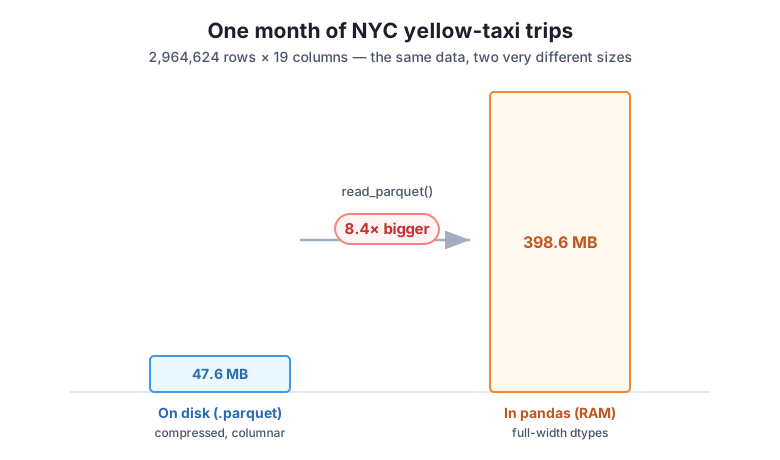
blow-up factor:  8.4x

There it is. A 47.6 MB file becomes 398.6 MB of live memory — an 8.4x expansion — for one month of one taxi color. That is not a bug, a leak, or a bad option somewhere. It’s the normal, expected gap between how data is stored and how pandas works with it, and understanding that gap is the whole point of this lesson.

Where the megabytes actually go#

“Nearly 400 MB” is a total. To do anything about it, you need to know which columns carry the weight. memory_usage(deep=True) returns a per-column breakdown, so let’s sort it and look at the heaviest few.

by_column = trips.memory_usage(deep=True) / 1024**2
print(by_column.sort_values(ascending=False).head(5).round(1))

store_and_fwd_flag      25.4
payment_type            22.6
fare_amount             22.6
congestion_surcharge    22.6
total_amount            22.6
dtype: float64

Two things stand out. First, most columns cost the same — right around 22.6 MB each. That’s not a coincidence: with 2.96 million rows, any column stored as an 8-byte float64 or int64 takes $2{,}964{,}624 \times 8$ bytes, which is 22.6 MB, every time. Second, a single tiny text column, store_and_fwd_flag, is the heaviest of all — even though it only ever holds the letter N or Y. Both of those clues point at the same culprit: dtypes. Pandas is spending 8 bytes on numbers that would fit in 1, and it’s spending a small fortune on two-letter strings. Let’s measure each.

Numbers: 8 bytes for a value that fits in 1#

Take payment_type. It’s a code: 1 for credit card, 2 for cash, and a handful of others. Let’s confirm its actual range, then compare storing it as a full-width int64 versus the narrowest integer type, int8.

payment = trips["payment_type"]
print("min / max value:", payment.min(), payment.max())

as_int64 = payment.astype("int64").memory_usage(deep=True, index=False) / 1024**2
as_int8  = payment.astype("int8").memory_usage(deep=True, index=False) / 1024**2

print(f"payment_type as int64: {as_int64:.1f} MB")
print(f"payment_type as int8:  {as_int8:.1f} MB")
print("values unchanged:", payment.astype("int8").astype("int64").equals(payment))

min / max value: 0 4
payment_type as int64: 22.6 MB
payment_type as int8:  2.8 MB
values unchanged: True

Every value in the column is between 0 and 4. An int8 holds any whole number from −128 to 127, so it stores these codes with room to spare — and the values come back exactly unchanged. Yet int64 reserves 8 bytes per value where int8 needs 1. That’s the 22.6 MB versus 2.8 MB you see: an 8x saving on this one column, for free, with zero information lost. float64 behaves the same way — 8 bytes per value — which is why every numeric column landed on 22.6 MB above.

Strings: a full Python object for every “N”#

Now the expensive one. store_and_fwd_flag holds only N or Y, so it should be nearly weightless. To see why it isn’t, let’s store it two ways: as ordinary Python string objects (object dtype, which is how every pandas version before 3.0 stored text by default), and as a category, which keeps one copy of each distinct value plus a compact integer code per row.

flag = trips["store_and_fwd_flag"]
print("distinct values:", flag.dropna().unique().tolist())

as_object   = flag.astype("object").memory_usage(deep=True, index=False) / 1024**2
as_category = flag.astype("category").memory_usage(deep=True, index=False) / 1024**2

print(f"as Python objects: {as_object:.1f} MB")
print(f"as category:       {as_category:.1f} MB")

distinct values: ['N', 'Y']
as Python objects: 160.5 MB
as category:       2.8 MB

Read those numbers again. The same two-letter column costs 160.5 MB as Python objects and 2.8 MB as a category — a 57x difference. When a column is object dtype, the array doesn’t hold the letters themselves; it holds a pointer to a full Python string object for every single row, and each of those objects carries heavy bookkeeping overhead. A one-character Python string takes about 50 bytes on its own — before you even count the 8-byte pointer to it. Multiply that by 2.96 million rows and a column of Ns and Ys balloons past 160 MB.

The category version, by contrast, stores the two distinct strings once and gives each row a tiny integer code pointing at them — which is exactly why it collapses to 2.8 MB. This per-value object overhead is the single biggest and most surprising memory cost in everyday pandas, and text columns are where large datasets quietly get out of hand.

Now scale it up: this is the wall#

One month fits in 398.6 MB. That’s uncomfortable on a laptop but survivable. The trouble is that CityFlow’s dashboard doesn’t run on one month — it runs on history. So let’s do the only arithmetic that matters: multiply the measured per-month cost by the number of months you’d actually want to analyze.

one_month_mb = trips.memory_usage(deep=True).sum() / 1024**2

for months in (1, 3, 6, 12):
    print(f"{months:2d} month(s): {one_month_mb * months / 1024:5.1f} GB in RAM")

 1 month(s):   0.4 GB in RAM
 3 month(s):   1.2 GB in RAM
 6 month(s):   2.3 GB in RAM
12 month(s):   4.7 GB in RAM

A single year of one taxi color needs 4.7 GB of RAM just to sit in a DataFrame — and that’s before you sort it, join it to the zone lookup, or make a working copy, each of which can transiently double the footprint. A laptop with 8 GB of RAM, much of it already claimed by the operating system and your browser, hits its ceiling somewhere around here. Add the green taxis, the for-hire vehicles, or a second year, and pd.read_parquet simply fails with a MemoryError — or, worse, your machine starts swapping to disk and everything crawls.

That is the memory wall: not a dramatic crash, but a hard limit you reach sooner than the modest file sizes suggest, because every gigabyte on disk becomes many in RAM. The good news is that nothing here is mysterious. You measured every number, and each one points at a lever — narrower dtypes, categories for text, loading only the columns and rows you need, processing in chunks, or moving off a single machine entirely. Those levers are the rest of this course.

Practice Exercises#

Exercise 1: Measure the whole frame yourself#

Load the month of trips with pd.read_parquet and print, in one script, the number of rows, the total in-memory size in MB from df.memory_usage(deep=True).sum(), and the file’s size on disk from os.path.getsize. Compute and print the blow-up factor (memory divided by disk size). Confirm you reproduce roughly the 8.4x figure from the lesson.

Exercise 2: Rank the columns by cost#

Build a per-column memory report: divide trips.memory_usage(deep=True) by 1024**2, sort it from largest to smallest, and print the result. Then, for the heaviest numeric column, print its min() and max(), and state which narrower integer type (int8, int16, or int32) would safely hold its full range.

Exercise 3: Put a number on the text cost#

Pick the store_and_fwd_flag column and measure it three ways with memory_usage(deep=True, index=False): as object, as its native dtype, and as category. Print all three sizes in MB and compute how many times larger the object version is than the category version. Explain in a sentence why converting a low-cardinality text column to category saves so much.

Summary#

You made the memory wall concrete. A real 47.6 MB month of NYC yellow-taxi trips — 2,964,624 rows across 19 columns — expands to 398.6 MB in pandas, an 8.4x blow-up you measured directly with df.memory_usage(deep=True). You traced that expansion to specific, measurable causes: full-width int64/float64 columns costing 8 bytes per value (22.6 MB each) where an int8 would need 1, and object strings costing 160.5 MB for a two-letter column because pandas keeps a full Python object per row. Finally, you multiplied one month by twelve and watched the total reach 4.7 GB — past the working limit of a typical laptop.

Key Concepts#

• In-memory size is not file size. Compressed columnar formats like Parquet are small on disk; pandas unpacks them into fixed-width, uncompressed arrays, and the gap here was 8.4x.
• df.memory_usage(deep=True) is the honest measuring tool. The deep=True flag makes it follow pointers to string objects instead of undercounting text columns.
• Numeric dtypes default to the widest safe type. int64 and float64 spend 8 bytes per value; many columns fit in int8/int16, but only if their real range allows it — check min() and max() before narrowing.
• object strings carry huge per-value overhead. Every row points to a separate Python string object, so low-cardinality text is far cheaper stored as category.
• The wall is reached by scale. A per-month footprint that looks fine multiplies with history until it crosses your machine’s RAM.

Why This Matters#

Every large-data technique in this course — right-sizing dtypes, using categories, selecting only the columns and rows you need, chunked processing, and eventually distributed engines like Spark — exists to manage the exact blow-up you just measured. Data engineers rarely fail because a file is too big to store; they fail because it’s too big to hold in memory the naive way. Knowing precisely where the megabytes go, and being able to prove it with a printed number rather than a hunch, is what turns “my kernel died” into a diagnosis and a fix. That measurement habit is the foundation the rest of CityFlow’s pipeline is built on.

Continue Building Your Skills#

You now know that the taxi data outgrows memory and why — full-width numbers and heavy object strings. In Lesson 2, you’ll turn that understanding into a repeatable skill: profiling a DataFrame’s memory in a disciplined way. You’ll build a reusable memory report that ranks every column by cost and dtype, learn to read df.info(memory_usage="deep") at a glance, and produce the kind of before-and-after profile that tells you which columns to attack first — the diagnostic step that comes before every reduction you’ll make for the rest of the course.