Lesson 2 - Profiling Memory & Dtypes

Welcome to Profiling Memory & Dtypes#

In Lesson 1 you watched a 50 MB month of NYC taxi trips balloon past 400 MB once it was a DataFrame, and you felt the memory wall as a real number. Feeling it is not the same as fixing it. Before your CityFlow team can shrink that footprint, you need to know which columns are eating the memory and why — because a fix that halves a 1 MB column is a rounding error, while the same trick on a 5 MB column is the whole game.

This lesson is about measurement. You will learn to ask a DataFrame exactly how many bytes it occupies, why the honest answer requires a “deep” count, how to rank columns from heaviest to lightest, and how much every common dtype costs per value. By the end you will have a small, reusable profile_memory() tool you can point at any taxi slice to get an instant breakdown. Every number below was measured on the real 200,000-row taxi sample your team uses for development.

By the end of this lesson, you will be able to:

• Read a DataFrame’s total memory with df.info(memory_usage="deep")
• Explain the difference between shallow and deep memory accounting, and when the gap matters
• Profile memory column by column to find the heaviest columns in a DataFrame
• Recall the byte-per-value cost of the common dtypes: the integer and float widths, datetime64, object, and category
• Write a reusable profile_memory() helper that ranks every column by its share of total memory

You only need pandas. Let’s measure the wall.

The One-Line Memory Readout#

The fastest way to see a DataFrame’s memory is df.info(). You have probably used it to check column names and null counts; it also reports a memory figure at the bottom. For an honest number, pass memory_usage="deep" — we will see in the next section exactly what “deep” buys you.

Load the CityFlow development sample and ask for the deep readout:

import warnings
warnings.filterwarnings("ignore")
import pandas as pd

taxi = pd.read_csv("https://datatweets.com/datasets/nyc-taxi/yellow_tripdata_sample.csv")
taxi.info(memory_usage="deep")

<class 'pandas.DataFrame'>
RangeIndex: 200000 entries, 0 to 199999
Data columns (total 10 columns):
 #   Column                 Non-Null Count   Dtype  
---  ------                 --------------   -----  
 0   tpep_pickup_datetime   200000 non-null  str    
 1   tpep_dropoff_datetime  200000 non-null  str    
 2   passenger_count        190489 non-null  float64
 3   trip_distance          200000 non-null  float64
 4   PULocationID           200000 non-null  int64  
 5   DOLocationID           200000 non-null  int64  
 6   payment_type           200000 non-null  int64  
 7   fare_amount            200000 non-null  float64
 8   tip_amount             200000 non-null  float64
 9   total_amount           200000 non-null  float64
dtypes: float64(5), int64(3), str(2)
memory usage: 22.5 MB

That last line — memory usage: 22.5 MB — is the whole DataFrame, index included. Three details are worth noticing right away. First, read_csv did not turn the two timestamp columns into dates: it left them as text (str), because parsing dates is something you ask for, not something it guesses. Second, passenger_count has only 190,489 non-null values out of 200,000 — the missing ones are why it is a float64 rather than an integer (pandas uses NaN, a float, to mark the gaps). Third, the str columns are already flagged as the odd ones out, and the rest of this lesson explains why they weigh the most.

Shallow vs Deep: What “deep” Actually Counts#

Why does info have a deep option at all? Because there are two honest ways to count a DataFrame’s memory, and they can disagree by a lot.

A DataFrame stores each column as an array. For a fixed-width column — an int64, a float64 — every value is the same size and lives directly inside that array, so counting is trivial: 200,000 values times 8 bytes each. But a plain object column (the classic way pandas holds Python strings) does not store the text inside the array. It stores an array of pointers — one 8-byte address per row — and each pointer aims at a separate Python string object living elsewhere in memory.

• Shallow accounting (deep=False, the default for memory_usage) counts only the array pandas holds directly. For an object column that is just the pointers: 8 bytes per row, no matter how long the strings are.
• Deep accounting (deep=True) follows every pointer and adds the size of the real object behind it. For text, that includes the actual characters.

The gap only appears when a column stores pointers to variable-size objects. To see it clearly, take the two timestamp columns and hold them the old-fashioned way, as a Python object column, then compare the two counts:

import warnings
warnings.filterwarnings("ignore")
import pandas as pd

taxi = pd.read_csv("https://datatweets.com/datasets/nyc-taxi/yellow_tripdata_sample.csv")

# Store the timestamps as classic Python string objects
legacy = taxi.copy()
legacy["tpep_pickup_datetime"] = legacy["tpep_pickup_datetime"].astype(object)
legacy["tpep_dropoff_datetime"] = legacy["tpep_dropoff_datetime"].astype(object)

shallow = legacy.memory_usage(deep=False).sum()
deep = legacy.memory_usage(deep=True).sum()
print(f"shallow: {shallow:>11,} bytes  ({shallow/1024/1024:5.1f} MB)")
print(f"deep:    {deep:>11,} bytes  ({deep/1024/1024:5.1f} MB)")
print(f"hidden:  {deep - shallow:>11,} bytes  ({(deep-shallow)/1024/1024:5.1f} MB)")

shallow:  16,000,132 bytes  ( 15.3 MB)
deep:     43,200,132 bytes  ( 41.2 MB)
hidden:   27,200,000 bytes  ( 25.9 MB)

Shallow accounting swears this DataFrame is 15.3 MB. Deep accounting reveals it is really 41.2 MB — the shallow count hid almost 26 MB of string data behind those pointers. If you had trusted the shallow number to plan how many months of taxi data fit in RAM, you would have been off by a factor of nearly three. This is exactly the trap the deep option exists to prevent, and it is why every measurement in this lesson uses deep=True.

Profiling Column by Column#

A single total tells you the size of the problem; it does not tell you where to aim. For that, drop the .sum() and keep the per-column series, then sort it so the heaviest columns rise to the top:

import warnings
warnings.filterwarnings("ignore")
import pandas as pd

taxi = pd.read_csv("https://datatweets.com/datasets/nyc-taxi/yellow_tripdata_sample.csv")

per_column = taxi.memory_usage(deep=True).sort_values(ascending=False)
print(per_column)

tpep_pickup_datetime     5400000
tpep_dropoff_datetime    5400000
passenger_count          1600000
trip_distance            1600000
PULocationID             1600000
DOLocationID             1600000
payment_type             1600000
fare_amount              1600000
tip_amount               1600000
total_amount             1600000
Index                        132
dtype: int64

Now the shape of the problem is obvious. The two timestamp columns weigh 5.4 MB each — every one of the other eight columns is a flat 1.6 MB. Those two text columns alone are 10.8 MB of the 22.5 MB total: nearly half the DataFrame lives in two columns. The Index line is a RangeIndex, which is basically free at 132 bytes because pandas stores it as “start, stop, step” rather than 200,000 separate numbers.

The figure below shows the same breakdown as a bar chart — the two text columns tower over the uniform numeric bars.

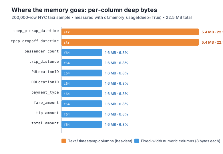
Why is every numeric column exactly 1.6 MB? Because 200,000 rows times 8 bytes per value is 1,600,000 bytes, and int64 and float64 both use 8 bytes per value. That uniformity is the clue to the next section: memory is dtype times row count, and once you know the per-value cost of each dtype, you can predict a column’s size before you even load it.

The Dtype Cost Table#

Every value in a fixed-width column costs a fixed number of bytes, set entirely by its dtype. Memorize this small table and you can estimate any column’s memory in your head — bytes per value times number of rows.

Notice the pattern: the number after the dtype name is its bit width, and bytes are bits divided by eight. int64 is 64 bits, so 8 bytes; int32 is 32 bits, so 4 bytes; int8 is 8 bits, so 1 byte. The default dtypes pandas picks — int64 and float64 — are the widest, most cautious choices. That caution is the opportunity you will exploit in Lesson 3.

Tie each taxi column to its dtype and cost:

• PULocationID, DOLocationID, payment_type are int64 — 8 bytes each — yet NYC has only 265 taxi zones and a handful of payment codes. These easily fit in an int16 (2 bytes) or even int8, so they are paying 4–8× too much.
• passenger_count, trip_distance, fare_amount, tip_amount, total_amount are float64 — 8 bytes each. Most carry only a couple of decimal places, so float32 (4 bytes) would halve them with room to spare.
• tpep_pickup_datetime, tpep_dropoff_datetime are text right now, which is why they are the heaviest columns. Parsed into datetime64 they drop to a flat 8 bytes per value — and parsing them is the right thing to do anyway, since you cannot do date math on a string.

The category row hints at the biggest win of all. A column like payment_type has only about five distinct values repeated across 200,000 rows. Storing it as a category keeps one tiny lookup table of those five values and replaces each row with a small integer code. Measure it:

import warnings
warnings.filterwarnings("ignore")
import pandas as pd

taxi = pd.read_csv("https://datatweets.com/datasets/nyc-taxi/yellow_tripdata_sample.csv")

as_int = taxi["payment_type"].memory_usage(deep=True)
as_cat = taxi["payment_type"].astype("category").memory_usage(deep=True)
print(f"payment_type as int64:    {as_int:>9,} bytes")
print(f"payment_type as category: {as_cat:>9,} bytes")
print(f"reduction: {as_int / as_cat:.1f}x")

payment_type as int64:    1,600,132 bytes
payment_type as category:   200,172 bytes
reduction: 8.0x

An 8× cut on one column, just by matching the dtype to the data. You will apply these moves systematically in the next lesson; for now the point is that profiling plus the cost table tells you precisely which columns are overpaying and by how much.

A Reusable profile_memory() Helper#

You will profile many taxi slices across this course, so wrap the workflow into a single function. A good profiler answers three questions per column at once: what dtype is it, how many bytes does it use, and what share of the total is that? Returning a sorted table makes the heaviest columns jump to the top.

import warnings
warnings.filterwarnings("ignore")
import pandas as pd

def profile_memory(df):
    """Return a per-column memory report: dtype, deep bytes, bytes/row, and % of total."""
    usage = df.memory_usage(deep=True).drop("Index")   # focus on the columns
    table = pd.DataFrame({
        "dtype": df.dtypes.astype(str),
        "bytes": usage,
    })
    table["bytes_per_row"] = (table["bytes"] / len(df)).round(1)
    table["pct_of_total"] = (100 * table["bytes"] / table["bytes"].sum()).round(1)
    return table.sort_values("bytes", ascending=False)

taxi = pd.read_csv("https://datatweets.com/datasets/nyc-taxi/yellow_tripdata_sample.csv")
print(profile_memory(taxi).to_string())

                         dtype    bytes  bytes_per_row  pct_of_total
tpep_pickup_datetime       str  5400000           27.0          22.9
tpep_dropoff_datetime      str  5400000           27.0          22.9
passenger_count        float64  1600000            8.0           6.8
trip_distance          float64  1600000            8.0           6.8
PULocationID             int64  1600000            8.0           6.8
DOLocationID             int64  1600000            8.0           6.8
payment_type             int64  1600000            8.0           6.8
fare_amount            float64  1600000            8.0           6.8
tip_amount             float64  1600000            8.0           6.8
total_amount           float64  1600000            8.0           6.8

One call now gives CityFlow a complete memory map. The pct_of_total column reads like a budget: the two timestamp columns claim 22.9% each — 45.8% between them — and the eight numeric columns split the rest evenly at 6.8% apiece. The bytes_per_row column confirms the cost table: 8.0 bytes for every numeric column, and 27.0 for the compact text columns. This is the exact starting point for a reduction plan: convert the timestamps to datetime64, narrow the integers, downcast the floats, and categorize the low-cardinality codes — each move now has a measured payoff attached.

Practice Exercises#

Exercise 1 — Prove the deep gap for yourself. Load the taxi sample, convert tpep_pickup_datetime to a plain object column with .astype(object), and print that single column’s memory both ways: .memory_usage(deep=False) and .memory_usage(deep=True). How many bytes per value does each report, and which number would you trust when planning RAM?

Exercise 2 — Find the heaviest column with a one-liner. Without sorting the whole table, return the name of the single heaviest column in the taxi DataFrame using memory_usage(deep=True). Then print how many megabytes it uses.

Exercise 3 — Estimate before you measure. Using only the dtype cost table, predict the bytes for a hypothetical 1,000,000-row column stored as int64, then as int16, then as category with 5 distinct values (assume 1 byte per code plus a negligible lookup). Then create such a column from the taxi sample and check your prediction with profile_memory().

Summary#

You learned to measure a DataFrame’s memory precisely instead of guessing. df.info(memory_usage="deep") gives the honest total; df.memory_usage(deep=True) gives it column by column. You saw why deep accounting matters — on the taxi timestamps held as Python objects, shallow counting hid nearly 26 MB behind 8-byte pointers, a 2.7× undercount. Profiling column by column showed the two text timestamp columns dominating at 5.4 MB each (45.8% of the DataFrame together), while every fixed-width numeric column sat at exactly 1.6 MB. The dtype cost table explained that uniformity — memory is bytes-per-value times row count — and showed that pandas’ default int64/float64 are the widest, most expensive choices. Finally, your profile_memory() helper packaged all of this into one call that ranks every column by its share of total memory.

Key Concepts#

• Shallow vs deep memory — shallow (deep=False) counts only the array pandas holds directly, which for object columns is just 8-byte pointers; deep (deep=True) follows those pointers to the real data. Always use deep=True.
• Per-column profiling — df.memory_usage(deep=True).sort_values(ascending=False) ranks columns from heaviest to lightest so you aim fixes where they pay off.
• The dtype cost table — the number in a dtype’s name is its bit width; bytes are bits over eight. int8=1, int16=2, int32=4, int64=8, float32=4, float64=8, datetime64=8 bytes per value; category replaces repeated values with tiny integer codes plus one shared lookup.
• Default dtypes are wide — pandas picks int64 and float64 to be safe, which is exactly why so many columns overpay and why profiling reveals easy wins.
• profile_memory(df) — a reusable report of dtype, bytes, bytes-per-row, and percent of total, sorted heaviest-first, that you can point at any taxi slice.

Why This Matters#

CityFlow cannot shrink a dataset it cannot see. Profiling turns “the taxi data is too big” into a ranked, numeric target list: these two columns are 46% of the memory, and here is the dtype each one should be. That is the difference between guessing and engineering. Every reduction technique in the rest of this course — dtype downcasting, categoricals, parsing dates, loading only the columns you need — is chosen and justified by the kind of measurement you just learned to take. Profile first, then fix; the numbers tell you what to touch and how much you will save.

Continue Building Your Skills#

You can now see exactly where a DataFrame’s memory goes and name the ideal dtype for every column. Lesson 3, Shrinking Memory with Smart Dtypes, turns that diagnosis into treatment. You will parse the timestamp columns into datetime64, downcast the wide integers to the narrowest width that safely fits NYC’s 265 zone IDs, convert the float64 money columns to float32, and turn the low-cardinality codes like payment_type into categoricals — measuring the DataFrame after each move with the very profile_memory() helper you just built. By the end you will have driven the taxi sample’s footprint down by a large, measured margin and produced the reduction plan this module has been building toward.