Lesson 3 - The Data Engineer's Toolkit

Welcome to The Data Engineer’s Toolkit#

In the first two lessons you felt the problem and learned to measure it: a 50 MB month of NYC taxi trips balloons past 400 MB in pandas, and you can now profile a DataFrame column by column to see exactly where that weight sits. At CityFlow, the mobility-analytics team you work on, knowing why the data is heavy is the easy half. The hard question your teammates keep asking is: what do I actually do about it?

This lesson is the map. Before you dive into any single technique, it helps to see all of them laid out in order, so you always know which tool to reach for and roughly what it costs you in effort. There are six techniques in this course, and they form a ladder from cheap-and-simple to heavy-and-complex. The whole philosophy of a good data engineer fits in one sentence: always try the cheapest fix first, and only climb the ladder when you have to.

By the end of this lesson, you will be able to:

• Name the six core techniques for handling data larger than memory, in cost order
• Explain what each technique does and when to reach for it
• Point to the module in this course where each one is taught
• Apply the cheapest technique yourself and measure a real memory reduction on the taxi data

You will not master any single tool here — each gets its own lessons later. Think of this as the table of contents you can hold in your head. Let’s walk the ladder.

The Ladder of Techniques#

When a dataset stops fitting comfortably in memory, there is a natural order in which to fight back. The techniques near the bottom of the ladder are cheap: a few lines of code, no new libraries, no change to how you think. The ones near the top are powerful but expensive: new tools, more moving parts, and often a different mental model. A skilled engineer climbs only as high as the problem forces them to.

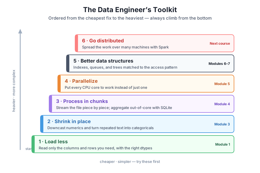
Here is each rung in turn.

1. Load less — the cheapest fix (Module 1)#

What it does: Instead of reading an entire file into memory and then throwing most of it away, you read only the columns and rows you actually need, and you tell pandas the right type for each column as it loads. A DataFrame you never build costs nothing.

When to reach for it: First. Always. Before any other trick, ask “do I even need all of this?” Most analyses touch a handful of columns out of dozens, and most files carry rows you will immediately filter out.

One-line preview: pd.read_csv(path, usecols=[...], dtype={...}) — you will do this in Lesson 4 and cut the taxi load by most of its size.

2. Shrink in place — make each value smaller (Module 3)#

What it does: Once the data is in memory, you make each value take fewer bytes. A whole-number column stored as a 64-bit integer often fits fine in 16 bits; a text column with only a few repeated values (like payment_type) becomes a compact categorical. Same data, a fraction of the RAM.

When to reach for it: When you have already loaded only what you need but the result is still too big — or when you want to keep a working DataFrame around for a while.

One-line preview: df["PULocationID"] = df["PULocationID"].astype("int16") and df["payment_type"] = df["payment_type"].astype("category"), covered in Module 3.

3. Process in chunks — never hold it all at once (Module 4)#

What it does: When even the frugal, shrunk version does not fit, you stop trying to hold the whole dataset in memory. You stream the file in pieces, do your work on one piece at a time, and keep only the running result. This is called out-of-core processing, and a small local database like SQLite can do the heavy aggregation for you.

When to reach for it: When the data is bigger than RAM no matter how you shrink it — the full taxi month, or a year of months stacked together.

One-line preview: for chunk in pd.read_csv(path, chunksize=100_000): ..., the heart of Module 4.

4. Parallelize — use every core (Module 5)#

What it does: Your laptop has several CPU cores, but plain pandas uses one. Parallelizing spreads the work across all of them, so a job that took four minutes on one core can finish in roughly one on four.

When to reach for it: When the data fits (perhaps in chunks) but the computation is the bottleneck — you are waiting on the CPU, not on memory.

One-line preview: splitting the work with multiprocessing and tools built on it, the focus of Module 5.

5. Better data structures — match the tool to the access pattern (Modules 6–7)#

What it does: Sometimes the fix is not “less data” but “smarter storage.” An index turns a slow full scan into an instant lookup; a queue streams work without ever materializing the whole backlog; a tree keeps sorted data searchable. Choosing the structure that fits how you actually read the data can beat any amount of raw shrinking.

When to reach for it: When the same big dataset is queried over and over, or when the access pattern (lookups, ranges, first-in-first-out) is predictable.

One-line preview: building indexes and streaming structures for repeated access, across Modules 6 and 7.

6. Go distributed — when one machine isn’t enough (the next course)#

What it does: Some datasets are too large for any single computer. Distributed frameworks like Apache Spark spread both the storage and the computation across a cluster of machines that work together as one.

When to reach for it: Last. Only when you have honestly exhausted the cheaper rungs and a single machine still cannot cope. Distribution buys enormous scale but costs you a cluster to manage, network overhead, and a new way of thinking.

One-line preview: a first taste of Spark closes this course, and the next course takes distribution seriously.

The Cheap Fixes Compound#

The most encouraging thing about this ladder is that the bottom rungs are not just cheap — they stack. Loading fewer columns and choosing smaller dtypes are independent wins, and they multiply together. Let’s prove it on the taxi sample, using nothing but rung one.

CityFlow’s reproducible teaching sample lives at https://datatweets.com/datasets/nyc-taxi/yellow_tripdata_sample.csv — 200,000 real trips, about 15 MB on disk. First, the naive way most people write it: read everything, accept the default types.

import pandas as pd

url = "https://datatweets.com/datasets/nyc-taxi/yellow_tripdata_sample.csv"

# The naive load: every column, default dtypes
naive = pd.read_csv(url)
naive_mb = naive.memory_usage(deep=True).sum() / 1e6

print("columns loaded:", len(naive.columns))
print("memory used:", round(naive_mb, 1), "MB")

columns loaded: 10
memory used: 23.6 MB

A 15 MB file already needs 23.6 MB of RAM. If you profile it column by column, the two timestamp columns, read as generic text, account for over 5 MB each — nearly half the total — and every whole-number column is stored in a wide 64-bit integer it does not need.

Now the frugal load. Suppose this analysis only cares about when a trip happened, how far it went, where it started, how it was paid for, and what it cost. That is five columns, not ten. We name them with usecols, hand pandas a smaller dtype for each numeric column, and parse the timestamp as a real datetime instead of text.

import pandas as pd

url = "https://datatweets.com/datasets/nyc-taxi/yellow_tripdata_sample.csv"

# The frugal load: only what we need, with the right types
cols = ["tpep_pickup_datetime", "trip_distance",
        "PULocationID", "payment_type", "total_amount"]
dtypes = {
    "trip_distance": "float32",
    "PULocationID": "int16",
    "payment_type": "int8",
    "total_amount": "float32",
}

frugal = pd.read_csv(
    url,
    usecols=cols,
    dtype=dtypes,
    parse_dates=["tpep_pickup_datetime"],
)
frugal_mb = frugal.memory_usage(deep=True).sum() / 1e6

print("columns loaded:", len(frugal.columns))
print("memory used:", round(frugal_mb, 1), "MB")
print("reduction:", round(23.6 / frugal_mb, 1), "x smaller")

columns loaded: 5
memory used: 3.8 MB
reduction: 6.2 x smaller

From 23.6 MB down to 3.8 MB — a 6.2x reduction, nearly 20 MB saved, and about 84% of the memory gone. No new library, no cluster, no chunking. Just two ideas from the bottom of the ladder, applied on the way in.

Notice why it compounds. Dropping five of the ten columns roughly halves the data. On top of that, the columns we kept got lighter: payment_type went from an 8-byte integer to a 1-byte one, PULocationID from 8 bytes to 2, and the timestamp became a true datetime instead of bulky text. Selection and shrinking are two separate levers, and pulling both together is what turns a 2x win into a 6x win.

That is the promise of the whole course in miniature: you rarely need the top of the ladder. Reach for the cheapest fix, measure the win, and climb only if the number is still too big.

Practice Exercises#

Exercise 1: Read the ladder#

Without looking back at the figure, list the six techniques in order from cheapest to heaviest, and for each one write a single phrase describing what it does. Then check yourself against the ladder above.

Exercise 2: Pick the right rung#

For each situation below, name the first technique you would reach for and say why:

1. You need only three of a file’s forty columns for a report.
2. Your frugal DataFrame fits in memory, but a groupby takes four minutes and one CPU core is pinned while the others sit idle.
3. The file is larger than your total RAM no matter which columns you drop.

Exercise 3: Measure your own compounding#

Adapt the frugal-load code to keep a different set of columns — say tpep_pickup_datetime, passenger_count, trip_distance, and fare_amount — with sensible small dtypes (passenger_count fits in int8, the money and distance columns in float32). Load both the naive and your frugal version, print each one’s memory in MB, and report the reduction factor. Did selection or dtype shrinking contribute more to your saving?

Summary#

This lesson gave you the map for the whole course. The six techniques for handling data larger than memory form a ladder ordered from cheapest to heaviest: load less, shrink in place, process in chunks, parallelize, use better data structures, and go distributed. Each rung has a clear job and a clear cost, and the guiding rule is to always try the cheapest fix first and climb only when forced. You then proved the payoff of the bottom rung on the real taxi sample, cutting a naive 23.6 MB load to 3.8 MB — a 6.2x reduction — using nothing but column selection and right-sized dtypes.

Key Concepts#

• The ladder — techniques ordered by cost: load less → shrink in place → chunk → parallelize → better data structures → distribute.
• Cheapest fix first — a decision procedure, not just a list; only climb a rung when the one below is genuinely insufficient.
• Cheap fixes compound — column selection and dtype shrinking are independent levers that multiply, turning a 2x win into 6.2x on the taxi sample.
• Where each lives — loading less is Module 1, shrinking is Module 3, chunking is Module 4, parallelizing is Module 5, data structures are Modules 6–7, and distribution opens the next course.

Why This Matters#

Real data-engineering work is full of the temptation to over-engineer — to reach for Spark or a cluster the moment a file feels big. This lesson gives you the antidote: a mental checklist that starts with two-line fixes and escalates deliberately. Knowing the order means you spend your effort where the data actually demands it, and the 6.2x reduction you measured on a single read_csv call is the everyday proof that most “big data” problems are solved long before you leave your laptop.

Continue Building Your Skills#

You have the map; now you start walking it. The very next lesson, Lesson 4: Loading Only What You Need, takes the bottom rung of the ladder — loading less — and turns the quick demo you just saw into a proper skill. You will learn exactly how usecols, nrows, and dtype behave on the taxi data, how to choose which columns to keep for a given question, and how to combine them into a loading pattern you will reuse in every lesson that follows. It is the cheapest technique in the toolkit, so it is the right place to begin doing real work.