Title here
Summary here
In the first three lessons you felt the memory wall and learned to read it. You watched a 50 MB taxi file expand past 400 MB in RAM, you profiled a DataFrame column by column to see exactly where the weight sits, and you surveyed the toolkit of techniques ahead. All of that was diagnosis. This lesson is your first treatment, and it happens to be the cheapest and most reliable one: stop loading data you were never going to use.
Here is the mindset shift. By default, pandas.read_csv reads every column, guesses a generous dtype for each (64-bit integers, 64-bit floats, strings for anything textual), and hands you the whole thing. That is convenient, but at CityFlow you almost never need all 19 taxi columns for a single task. A tip-percentage report needs the fare, the tip, and maybe the pickup time. A trips-per-zone chart needs the pickup location and nothing else. Every column you read but ignore is RAM you paid for and threw away.
In this lesson you’ll fix that at the source. You’ll tell the reader which columns to bring back (usecols), what small type each should be (dtype), which text columns are really dates (parse_dates), and how to grab a quick sample without loading the file (nrows). Then you’ll do the same trick for parquet, where column selection is even more powerful because it happens on disk before a single unwanted byte is read. Every number below was measured on the real NYC taxi data.
By the end of this lesson, you will be able to:
usecols= to read only the columns a task needs and measure the memory saved.dtype= at read time so pandas uses small integers, 32-bit floats, and category instead of its wasteful defaults.parse_dates= and take a quick look at a file with nrows=.columns= so unused columns never leave the disk.Throughout this module CityFlow works with a reproducible slice of the NYC Taxi & Limousine Commission’s public trip records: 200,000 real yellow-taxi trips with the ten columns most teams actually use. It lives at:
https://datatweets.com/datasets/nyc-taxi/yellow_tripdata_sample.csv (the CSV sample, ~15 MB on disk)https://datatweets.com/datasets/nyc-taxi/taxi_zone_lookup.csv (the 265-zone lookup, for later joins)For the “now scale it up” moments we also reach for a full month as parquet:
https://d37ci6vzurychx.cloudfront.net/trip-data/yellow_tripdata_2024-01.parquet (~2.96 million trips)The sample keeps these columns: tpep_pickup_datetime, tpep_dropoff_datetime, passenger_count, trip_distance, PULocationID, DOLocationID, payment_type, fare_amount, tip_amount, total_amount. In the examples below the variable CSV points at the sample and PARQUET at the full month.
# gate: skip
CSV = "https://datatweets.com/datasets/nyc-taxi/yellow_tripdata_sample.csv"
PARQUET = "https://d37ci6vzurychx.cloudfront.net/trip-data/yellow_tripdata_2024-01.parquet"First, the honest baseline. We read the whole sample the default way and measure it. Throughout this lesson we use one small helper so every measurement is apples-to-apples:
import warnings
warnings.filterwarnings("ignore")
import pandas as pd

CSV = "yellow_tripdata_sample.csv"

def mb(df):
    """Total memory of a DataFrame in MB, counting real string sizes."""
    return df.memory_usage(deep=True).sum() / 1024**2

naive = pd.read_csv(CSV)
print(naive.dtypes)
print("Naive read:", round(mb(naive), 1), "MB")
tpep_pickup_datetime str
tpep_dropoff_datetime str
passenger_count float64
trip_distance float64
PULocationID int64
DOLocationID int64
payment_type int64
fare_amount float64
tip_amount float64
total_amount float64
Naive read: 22.5 MBTwenty-two and a half megabytes for a file that is about fifteen on disk. Look at the dtypes and you can see where the money went. The two datetime columns came in as strings because a CSV has no idea they are dates. The integer columns are int64 — eight bytes each — even though payment_type only ever holds a handful of small codes. The floats are all float64. Nothing here is wrong, exactly; it’s just pandas defaulting to the biggest, safest type for everything because you didn’t tell it otherwise.
deep=True is not optional here
We call memory_usage(deep=True) rather than the default memory_usage(). The shallow version only counts the pointer array for text columns, not the actual characters, so it can under-report a string-heavy DataFrame by a wide margin. When you are trying to decide what to cut, you want the real number. This is exactly the profiling habit from Lesson 2.
usecols: read only the columns you needSuppose the task is a fare-and-tip summary by pickup time. You need six columns, not ten. The usecols= argument tells read_csv to bring back only those — the rest are never parsed into memory at all.
import warnings
warnings.filterwarnings("ignore")
import pandas as pd

CSV = "yellow_tripdata_sample.csv"

def mb(df):
    return df.memory_usage(deep=True).sum() / 1024**2

wanted = ["tpep_pickup_datetime", "passenger_count", "trip_distance",
          "PULocationID", "payment_type", "fare_amount"]

subset = pd.read_csv(CSV, usecols=wanted)
print("usecols only:", round(mb(subset), 1), "MB")
usecols only: 12.8 MBDropping four columns took us from 22.5 MB to 12.8 MB — a 43% cut for the price of one keyword argument, and we haven’t touched dtypes yet. This is the highest-leverage move in the whole lesson because it is pure subtraction: a column you don’t read costs exactly nothing. Before you optimize the types of a column, ask whether you need the column at all.
usecols also accepts a callable if you’d rather describe the columns than list them — for example usecols=lambda c: not c.startswith("DO") to skip every drop-off field. And it happily reorders: pass the names in any order and pandas returns them in the file’s order, so you don’t have to memorize the layout.
dtype: stop paying for 64 bits you don’t useNow the second lever. Even the six columns we kept are stored in oversized types. payment_type is a code from 1 to 6; it does not need 64 bits. PULocationID ranges over 265 zones; a 16-bit integer covers it four times over. Fares fit comfortably in a 32-bit float. We can declare all of this at read time with dtype=, and parse the pickup timestamp as a real datetime while we’re at it.
import warnings
warnings.filterwarnings("ignore")
import pandas as pd

CSV = "yellow_tripdata_sample.csv"

def mb(df):
    return df.memory_usage(deep=True).sum() / 1024**2

wanted = ["tpep_pickup_datetime", "passenger_count", "trip_distance",
          "PULocationID", "payment_type", "fare_amount"]

small_dtypes = {
    "passenger_count": "Int8",     # nullable small int (some rows are blank)
    "trip_distance": "float32",
    "PULocationID": "int16",       # 265 zones fit easily
    "payment_type": "int8",        # a handful of codes
    "fare_amount": "float32",
}

lean = pd.read_csv(
    CSV,
    usecols=wanted,
    dtype=small_dtypes,
    parse_dates=["tpep_pickup_datetime"],
)
print(lean.dtypes)
print("usecols + dtype + parse_dates:", round(mb(lean), 1), "MB")
tpep_pickup_datetime datetime64[us]
passenger_count Int8
trip_distance float32
PULocationID int16
payment_type int8
fare_amount float32
usecols + dtype + parse_dates: 4.0 MBFour megabytes. From the 22.5 MB naive read, that is 18.5 MB saved — the DataFrame is 82% smaller, and it happened entirely at read time. No .astype() pass afterward, no temporary double-memory moment where the big version and the small version both exist. The reader built the compact frame directly.
A couple of details worth noticing. We used Int8 (capital I) for passenger_count because a few rows are blank in the raw data, and the capital-I nullable integer type can hold a missing value where plain int8 cannot. And parse_dates turned the pickup column from a string into a real datetime64, which is both smaller and immediately usable for time filtering — a topic you’ll lean on in the next module.
Downcast on purpose, not by reflex
Small dtypes have limits, and silently overflowing one corrupts your data. An int8 only reaches 127; an int16 reaches 32,767. Before you assign a type, check the column’s real range with df["col"].min() and df["col"].max(), or use pd.to_numeric(s, downcast="integer") to let pandas pick the smallest safe integer type for you. Zone IDs and payment codes are safe forever; a running total or a row counter is not.
category type for repeated valuesThere’s one more dtype worth calling out on its own, because it can be dramatic. When a column has only a few distinct values repeated across millions of rows — payment_type, store_and_fwd_flag, a borough name — the category type stores each distinct value once and keeps a compact code per row.
import warnings
warnings.filterwarnings("ignore")
import pandas as pd

CSV = "yellow_tripdata_sample.csv"

def mb(df):
    return df.memory_usage(deep=True).sum() / 1024**2

as_int = pd.read_csv(CSV, usecols=["payment_type"])
as_cat = pd.read_csv(CSV, usecols=["payment_type"], dtype={"payment_type": "category"})

print("payment_type as int64:   ", round(mb(as_int), 3), "MB",
      "(", as_int["payment_type"].nunique(), "distinct values )")
print("payment_type as category:", round(mb(as_cat), 3), "MB")
payment_type as int64: 1.526 MB ( 5 distinct values )
payment_type as category: 0.191 MBFive distinct values across 200,000 rows, and category stores that in about an eighth of the space. On the full-month file, where a text column like store_and_fwd_flag repeats “N” or “Y” across millions of rows, the effect is even larger. The rule of thumb: if a column has far fewer distinct values than rows, reach for category.
nrows: peek without loadingBefore you commit to a plan, you often just want to see the file — the column names, a few example rows, the shape of the values. Reading all 200,000 rows to look at five of them is wasteful. nrows= reads only the first N rows and stops.
import warnings
warnings.filterwarnings("ignore")
import pandas as pd

CSV = "yellow_tripdata_sample.csv"

peek = pd.read_csv(CSV, nrows=5)
print("peek shape:", peek.shape)
print(peek[["passenger_count", "trip_distance", "fare_amount"]])
peek shape: (5, 10)
passenger_count trip_distance fare_amount
0 2.0 17.14 70.0
1 1.0 2.49 13.5
2 2.0 1.84 10.0
3 1.0 3.60 23.3
4 1.0 0.04 3.7Five rows, instant. This is how you should start every session with an unfamiliar file: nrows=5 (or nrows=1000 for a real feel of the value ranges) to learn the columns and decide your usecols and dtype plan — then do the full read. It turns “let me load this 2 GB file and wait” into a one-second glance.
Here is the whole read-time story on the CSV sample, measured on the real data:
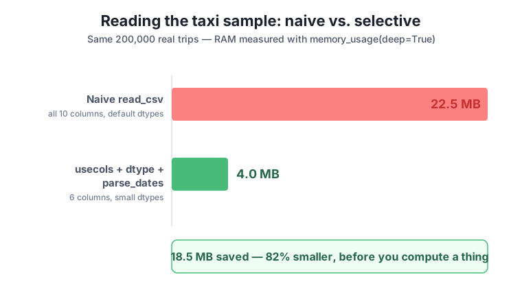
read_csv brings all ten columns back with default 64-bit types and string dates for 22.5 MB. Selecting six columns with usecols, declaring small dtypes, and parsing the pickup date brings the same task down to 4.0 MB — an 82% reduction paid entirely at read time, with no post-processing pass.The order of operations matters: subtract columns first (usecols), then shrink what remains (dtype), then parse dates (parse_dates). Column subtraction is free and often the biggest single win; dtype shrinking multiplies the savings on the columns you keep.
CSV is a row-oriented text format, so even with usecols pandas still has to scan across every row and skip the columns you didn’t ask for. Parquet is different. It stores each column separately (columnar layout), which means selecting columns can happen on disk: the reader seeks straight to the columns you named and never touches the rest. Passing columns= to read_parquet is that pushdown.
Here is the full month — nearly three million trips — read two ways:
import warnings
warnings.filterwarnings("ignore")
import pandas as pd

PARQUET = "yellow_2024_01.parquet"

def mb(df):
    return df.memory_usage(deep=True).sum() / 1024**2

full = pd.read_parquet(PARQUET)
print("Full parquet:", full.shape, "->", round(mb(full), 1), "MB")

want = ["tpep_pickup_datetime", "trip_distance", "PULocationID", "fare_amount"]
selected = pd.read_parquet(PARQUET, columns=want)
print("Four columns: ", selected.shape, "->", round(mb(selected), 1), "MB")
Full parquet: (2964624, 19) -> 398.6 MB
Four columns: (2964624, 4) -> 79.2 MBThe full month is the 398 MB memory wall from Lesson 1 in the flesh: 19 columns times 2.96 million rows. Ask for the four columns your task actually uses and you get 79 MB — an 80% cut — and, crucially, the other 15 columns were never read off the disk at all. With a CSV, usecols saves memory but the reader still had to walk past the unwanted columns; with parquet, columns= saves the disk read and the memory. This is a big part of why data engineers reach for parquet once files get large, a theme this course returns to.
Column pushdown is a preview of a bigger idea
columns= on parquet is your first taste of predicate and projection pushdown — the principle that the cheapest work is the work you never do because you told the storage layer not to. Later in the course you’ll see the same idea let a query engine skip whole row groups based on a filter, and let a distributed engine read only the file partitions a query needs. Same instinct, larger scale: describe what you need precisely and let the reader avoid the rest.
CityFlow wants a tip-behavior report. It needs tpep_pickup_datetime, payment_type, fare_amount, tip_amount, and total_amount — and nothing else. Write a single read_csv call against the sample that returns exactly those five columns, parses the pickup time as a datetime, and uses category for payment_type and float32 for the three money columns. Print the resulting dtypes and the total memory with memory_usage(deep=True).
Hint
Combine all four levers in one call: usecols=[...], parse_dates=["tpep_pickup_datetime"], and a dtype={...} dict that maps payment_type to "category" and each money column to "float32". Reuse the mb(df) helper from the lesson to print the megabytes. Compare it against a naive read_csv(CSV, usecols=the_same_five) to see how much the dtypes alone bought you.
Before trusting PULocationID as int16 and payment_type as int8, verify the values actually fit. Read just those two columns with usecols, then print the .min() and .max() of each. Confirm that PULocationID stays within the int16 range (−32,768 to 32,767) and payment_type within the int8 range (−128 to 127). Then explain in a comment why total_amount would be a bad candidate for int8.
Hint
pd.read_csv(CSV, usecols=["PULocationID", "payment_type"]) gets you the two columns cheaply. For each, df["col"].min() and df["col"].max() reveal the range. The lesson’s tip callout has the type limits. For the comment: int8 tops out at 127, and plenty of taxi fares plus tips and tolls exceed that — and an integer type would throw away the cents entirely.
Read the same four columns — tpep_pickup_datetime, trip_distance, PULocationID, fare_amount — two ways: from the CSV sample with usecols=, and from the full-month parquet with columns=. Print the shape and mb(...) of each. Note that the parquet has far more rows, so it uses more RAM in total; the point of the exercise is to observe that both formats let you name the columns, but only parquet avoids reading the unnamed ones off disk.
Hint
For the CSV, pd.read_csv(CSV, usecols=want); for parquet, pd.read_parquet(PARQUET, columns=want), where want is the same four-name list. The row counts differ (200,000 vs. ~2.96 million), so compare the ratio of memory to rows, or simply reflect on which read had to touch the columns it discarded. There is no single “right” number here — the goal is to internalize the difference between row-oriented and columnar selection.
You took the first concrete step down from the memory wall, and it cost almost nothing. By reading only the columns a task needs (usecols), declaring small dtypes at read time (dtype, including category for repeated values), parsing dates (parse_dates), and peeking with nrows, you cut the same 200,000-trip sample from a naive 22.5 MB to 4.0 MB — an 82% reduction — with no post-processing pass. On parquet, columns= pushed selection down to the disk and shrank a full-month read from 398.6 MB to 79.2 MB while never touching the unused columns. Every one of those numbers came from running the code on the real NYC taxi data.
usecols= — read only named columns; a column you don’t read costs zero. Highest-leverage single change (43% here, before any dtype work).dtype= — override pandas’ generous 64-bit defaults with int8/int16, float32, nullable Int8, and category. Check a column’s real range first so you never overflow a small type.parse_dates= — turn string date columns into compact, usable datetime64 at read time instead of an .astype() pass afterward.nrows= — load the first N rows to inspect a file’s structure and value ranges before committing to a full read.columns= — columnar pushdown: the reader seeks only to the named columns on disk and skips the rest entirely, saving both the read and the RAM.At CityFlow the pipeline runs on a schedule, on shared hardware, against files that only grow. A read that fits in 4 MB where the naive version needed 22 MB is not just tidier — it is the difference between a job that survives next quarter’s data volume and one that starts crashing with MemoryError at 3 a.m. Loading only what you need is the habit that makes every later technique — chunking, out-of-core processing, distribution — start from a smaller, saner baseline. And the underlying instinct, “describe exactly what you need and let the reader skip the rest,” scales all the way up to the query engines you’ll meet later in this course.
You now have every measurement tool from this module in hand: you can profile a DataFrame’s memory column by column, and you can cut that memory at read time with usecols, dtype, parse_dates, and parquet’s columns=. In Lesson 5, the module’s guided profiling project, you’ll put it all together on the full NYC taxi dataset — profile every column of the 398 MB month, decide the smallest safe type for each, and produce a concrete reduction plan and an optimized read recipe that the rest of the course will build on. Bring the mb() helper; you’re about to use it in anger.
Keep DATATWEETS free. Help fund practical data, AI, and engineering lessons for learners worldwide.
