Lesson 5 - Guided Project: Profile the NYC Taxi Data

Welcome to the Guided Project#

For four lessons you have been building instruments: you measured the memory wall, learned to profile a DataFrame column by column, surveyed the data engineer’s toolkit, and practiced loading only what you need. Now you put all of it to work at once, on the real thing.

You are still a data engineer at CityFlow. Before the team commits to a loading strategy for the public taxi dashboard, someone has to answer a plain question: exactly how heavy is one month of trips, where does the weight sit, and how much of it can we cut without throwing away anything the dashboard needs? That someone is you, and the deliverable is a reduction plan — a short, evidence-backed document that says which columns to drop, which dtypes to change, and what the memory will be afterward. In Module 3 you will execute this exact plan against the pipeline; today you produce it.

You will work the full month — 2,964,624 real trips — not a sample. Every number below is measured, and you will reproduce every one of them.

By the end of this project, you will be able to:

• Load the full month of NYC taxi data and measure its real disk-versus-memory blow-up factor
• Build a per-column memory table that ranks every column by how much RAM it costs
• Identify the heaviest columns and name a cheaper representation for each one, with an estimated saving
• Catch concrete data-quality problems using nothing but the profile you built
• Assemble a reduction plan and apply it, measuring the real before-and-after memory

The dataset#

Everything runs on New York City’s public-domain Yellow Taxi trip records, published by the NYC Taxi & Limousine Commission (TLC). The full month you will profile is the official TLC Parquet file:

• Full month, 2,964,624 rows, 19 columns: https://d37ci6vzurychx.cloudfront.net/trip-data/yellow_tripdata_2024-01.parquet

CityFlow also mirrors a smaller 200,000-row teaching sample and the zone lookup dimension for quick experiments:

• Teaching sample (10 columns): https://datatweets.com/datasets/nyc-taxi/yellow_tripdata_sample.csv
• Zone lookup (265 zones): https://datatweets.com/datasets/nyc-taxi/taxi_zone_lookup.csv

This project uses the full month, because the whole point is to feel the real scale.

Stage 1: Load and measure the blow-up#

Start with the number that motivates the entire module: how much bigger is this data in RAM than it is on disk? Parquet stores columns compressed, so the file is small; pandas has to decompress and materialize every value in memory. Measure both sides and divide.

import warnings
warnings.filterwarnings("ignore")
import os
import urllib.request
import pandas as pd

# The full month of real NYC Yellow Taxi trips (public-domain TLC data).
url = "https://d37ci6vzurychx.cloudfront.net/trip-data/yellow_tripdata_2024-01.parquet"
path = "yellow_tripdata_2024-01.parquet"
if not os.path.exists(path):
    urllib.request.urlretrieve(url, path)

disk_mb = os.path.getsize(path) / 1024**2
taxi = pd.read_parquet(path)
mem_mb = taxi.memory_usage(deep=True).sum() / 1024**2

print(f"rows on file:   {len(taxi):,}")
print(f"columns:        {taxi.shape[1]}")
print(f"size on disk:   {disk_mb:6.1f} MB")
print(f"size in memory: {mem_mb:6.1f} MB")
print(f"blow-up factor: {mem_mb / disk_mb:6.1f}x")

rows on file:   2,964,624
columns:        19
size on disk:     47.6 MB
size in memory:  398.6 MB
blow-up factor:    8.4x

There it is: a 47.6 MB file that becomes 398.6 MB the instant pandas holds it — an 8.4x blow-up. Two forces drive that gap. Parquet’s columnar compression is doing real work on disk, and pandas defaults to wide, uniform dtypes (mostly 64-bit) in memory. The rest of this project is about clawing that 398.6 MB back down.

Notice we used memory_usage(deep=True). The deep=True matters: without it, pandas reports only the pointer array for text columns, not the actual characters, and undercounts. Always measure deep when the answer will inform a decision.

Stage 2: Profile the memory per column#

A single total tells you how much; it does not tell you where. To spend your effort well, you need the weight broken down column by column. This is the profile_memory idea from Lesson 2 — for each column, record its dtype, its deep memory in megabytes, and its share of the total, then sort so the heaviest rises to the top.

def profile_memory(df):
    usage = df.memory_usage(deep=True)
    usage = usage.drop("Index")
    total = usage.sum()
    report = pd.DataFrame({
        "dtype": [str(df[c].dtype) for c in df.columns],
        "memory_mb": (usage / 1024**2).round(2).values,
        "pct_of_total": (100 * usage / total).round(1).values,
    }, index=df.columns)
    return report.sort_values("memory_mb", ascending=False)

profile = profile_memory(taxi)
print(profile.head(8).to_string())

                         dtype  memory_mb  pct_of_total
store_and_fwd_flag         str      25.42           6.4
payment_type             int64      22.62           5.7
fare_amount            float64      22.62           5.7
congestion_surcharge   float64      22.62           5.7
total_amount           float64      22.62           5.7
improvement_surcharge  float64      22.62           5.7
tolls_amount           float64      22.62           5.7
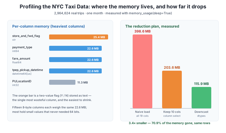
tip_amount             float64      22.62           5.7

Read this carefully, because the shape of it is the whole insight. The single heaviest column is store_and_fwd_flag at 25.42 MB — and it is a text column holding a one-letter flag. Right behind it sits a long tie: fifteen different columns each weighing exactly 22.62 MB (5.7% apiece). That is not a coincidence. Every one of them is an 8-byte type — int64, float64, or datetime64 — and $2{,}964{,}624 \text{ rows} \times 8 \text{ bytes} \approx 22.6\text{ MB}$. When storage is uniform, cost is uniform.

So the heaviest columns fall into two clear buckets:

1. One oversized text column — store_and_fwd_flag (25.42 MB), holding just Y / N.
2. A wall of 8-byte columns — payment_type, fare_amount, tip_amount, total_amount, the two datetime columns, and the surcharge fields — each 22.62 MB, many holding values that are far smaller than 64 bits allow.

Those two buckets are where every megabyte of savings will come from.

Stage 3: Spot the reductions (and the dirty data)#

Now turn each heavy column into a decision. For every one, the question is the same: what is the smallest representation that still holds every real value? Measure the answer rather than guessing it.

The text flag becomes a category#

store_and_fwd_flag records whether a trip was stored in the meter before being forwarded — in practice, Y or N. Storing two distinct strings once and pointing each row at them (a category) is far cheaper than storing the character data 2.96 million times.

flag = taxi["store_and_fwd_flag"]
print("store_and_fwd_flag values:", list(flag.dropna().unique()))
as_text = flag.memory_usage(deep=True) / 1024**2
as_cat = flag.astype("category").memory_usage(deep=True) / 1024**2
print(f"as text:     {as_text:5.1f} MB")
print(f"as category: {as_cat:5.1f} MB")

pay = taxi["payment_type"]
print("payment_type range:", int(pay.min()), "to", int(pay.max()))
print(f"as int64: {pay.memory_usage(deep=True)/1024**2:5.1f} MB")
print(f"as int8:  {pay.astype('int8').memory_usage(deep=True)/1024**2:5.1f} MB")

store_and_fwd_flag values: ['N', 'Y']
as text:      25.4 MB
as category:   2.8 MB
payment_type range: 0 to 4
as int64:  22.6 MB
as int8:    2.8 MB

Two columns, two easy wins. Converting the flag from text to category drops it from 25.4 MB to 2.8 MB — a 22.6 MB saving from a two-value column. And payment_type only ever holds the integers 0 through 4, which fit comfortably in a single signed byte (int8, range −128 to 127). Downcasting int64 to int8 takes it from 22.6 MB to 2.8 MB. The same logic applies to the money columns: fare_amount, tip_amount, and total_amount are float64 but hold dollar amounts that float32 represents fine, halving each from 22.6 MB to about 11.3 MB. And PULocationID / DOLocationID are zone IDs from 1 to 265, which fit in an int16 (up to 32,767) at half their current size.

A profile also catches dirty data#

Profiling forces you to look at ranges and extremes, and that is exactly where real-world data betrays itself. Before you trust any of these columns, check whether their values even make sense.

pickup = taxi["tpep_pickup_datetime"]
print("earliest pickup:", pickup.min())
print("latest pickup:  ", pickup.max())
in_month = (pickup >= "2024-01-01") & (pickup < "2024-02-01")
print("trips dated outside January 2024:", (~in_month).sum())
neg = (taxi["fare_amount"] < 0).sum()
print("trips with a negative fare_amount:", f"{neg:,}")
print("most negative fare_amount:", taxi["fare_amount"].min())

earliest pickup: 2002-12-31 22:59:39
latest pickup:   2024-02-01 00:01:15
trips dated outside January 2024: 18
trips with a negative fare_amount: 37,448
most negative fare_amount: -899.0

This is a January 2024 file, yet its earliest pickup is timestamped 2002-12-31 — more than two decades early. Eighteen trips fall outside the month entirely, and a startling 37,448 trips carry a negative fare_amount, the worst being −$899.00. None of these are your bug; they are genuine artifacts of a meter feed at city scale — miscalibrated clocks, and refunds or adjustments booked as negative fares. You are not fixing them today. You are recording them, because a plan that ignores them would quietly poison every downstream average the dashboard shows.

The figure below shows both halves of the profile — where the memory sits, and how far the plan will take it.

Stage 4: The reduction plan#

You now have everything you need to write the plan. State it in plain language first, then apply it and measure the result — because a plan whose savings you have not measured is only a hope.

CityFlow taxi-data reduction plan (January 2024):

• Drop the columns the dashboard does not use. Keep only the ten columns the CityFlow sample already standardizes on — the two datetime columns, passenger_count, trip_distance, PULocationID, DOLocationID, payment_type, fare_amount, tip_amount, total_amount — and drop the other nine (the surcharge and flag columns) at load time. Expected: roughly halves the memory before any dtype work.
• Downcast the survivors to the smallest dtype that fits. payment_type to int8; PULocationID and DOLocationID to int16; passenger_count, trip_distance, and the three money columns to float32. Expected: cuts the kept columns roughly in half again.
• Note the data-quality work for later. The 18 out-of-range dates and 37,448 negative fares are recorded here and will be filtered in the cleaning stage of the pipeline, not silently dropped now.
• Expected memory after: comfortably under a third of the naive load.

Now apply the first two points and measure. Selecting columns is done right in read_parquet (the columns= argument you met in Lesson 4), so the dropped columns never enter memory at all.

naive_mb = taxi.memory_usage(deep=True).drop("Index").sum() / 1024**2

keep = [
    "tpep_pickup_datetime", "tpep_dropoff_datetime", "passenger_count",
    "trip_distance", "PULocationID", "DOLocationID", "payment_type",
    "fare_amount", "tip_amount", "total_amount",
]
slim = pd.read_parquet(path, columns=keep)
selected_mb = slim.memory_usage(deep=True).drop("Index").sum() / 1024**2

slim = slim.astype({
    "payment_type": "int8",
    "PULocationID": "int16",
    "DOLocationID": "int16",
    "passenger_count": "float32",
    "trip_distance": "float32",
    "fare_amount": "float32",
    "tip_amount": "float32",
    "total_amount": "float32",
})
reduced_mb = slim.memory_usage(deep=True).drop("Index").sum() / 1024**2

print(f"naive load (19 columns, wide dtypes): {naive_mb:6.1f} MB")
print(f"after keeping 10 columns:             {selected_mb:6.1f} MB")
print(f"after downcasting dtypes:             {reduced_mb:6.1f} MB")
print(f"final size is {naive_mb / reduced_mb:.1f}x smaller "
      f"({100 * (1 - reduced_mb / naive_mb):.0f}% saved)")

naive load (19 columns, wide dtypes):  398.6 MB
after keeping 10 columns:              203.6 MB
after downcasting dtypes:              115.9 MB
final size is 3.4x smaller (71% saved)

The plan holds up under measurement. Dropping the nine unused columns takes the DataFrame from 398.6 MB to 203.6 MB — almost exactly half, because most of those columns were full-width 8-byte fields. Downcasting the ten survivors then drops it again to 115.9 MB. The full month of taxi trips, all 2,964,624 rows intact, now fits in 115.9 MB instead of 398.6 MB — 3.4x smaller, 71% of the memory gone, and you did not discard a single row.

That is the deliverable. In Module 3 you will apply this same plan inside the loading step of the CityFlow pipeline, and add the data-quality filters you flagged in Stage 3. For now, you have turned a vague worry (“the file is big”) into a concrete, measured, reproducible plan.

Practice Exercises#

These extend the profile you just built. The taxi DataFrame is the full month loaded in Stage 1.

Exercise 1. The two datetime columns, tpep_pickup_datetime and tpep_dropoff_datetime, each cost 22.62 MB. Unlike payment_type, they cannot be downcast to a tiny integer — but they can be dropped if the dashboard only needs the trip duration. Compute a new float32 column, trip_minutes, as the difference between dropoff and pickup in minutes, then report how much memory that single float32 column uses compared to the 45.2 MB the two datetime columns cost together.

Exercise 2. In Stage 3 you found 37,448 trips with a negative fare_amount. Extend the data-quality check: count how many trips have a trip_distance of exactly 0, and how many have a passenger_count of 0. Print each count and its percentage of all 2,964,624 rows, so the plan can note them alongside the negative fares.

Exercise 3. Your Stage 4 plan cut the memory to 115.9 MB. Push it one step further by adding store_and_fwd_flag to the kept columns and storing it as a category, and by converting payment_type to a category as well (its five values behave like labels, not numbers). Re-measure the total memory of this eleven-column version and compare it to the 115.9 MB ten-column version — is the extra column worth its cost?

Summary#

You profiled a real month of NYC taxi data end to end and produced a measured reduction plan. The naive load of 2,964,624 rows cost 398.6 MB — an 8.4x blow-up over the 47.6 MB file. A per-column profile showed one oversized text flag (25.42 MB) and a wall of identical 8-byte columns (22.62 MB each). By naming a cheaper representation for each heavy column, dropping the nine columns the dashboard does not use, and downcasting the ten that remain, you cut the DataFrame to 115.9 MB — 3.4x smaller, 71% saved — while keeping every row. Along the way the profile surfaced genuine dirty data: a pickup timestamp from 2002, 18 trips outside the month, and 37,448 negative fares.

Key Concepts#

• Blow-up factor — the ratio of in-memory size to on-disk size. For this file it is 8.4x, driven by Parquet compression on disk and pandas’ wide default dtypes in memory.
• Per-column memory profile — ranking columns by memory_usage(deep=True) reveals that a few columns dominate; uniform 8-byte dtypes make many columns cost an identical amount.
• Cheaper representations — text with few distinct values becomes category; small integers downcast to int8 / int16; wide floats become float32; unused columns are dropped at load time.
• Profiling as data-quality triage — inspecting each column’s extremes catches impossible values (a 2002 date, a negative fare) before they corrupt downstream results.
• A measured plan — every expected saving is confirmed with a real before-and-after number, not estimated and hoped for.

Why This Matters#

Real pipelines do not shrink data by folklore; they shrink it by profile. The habit you practiced here — measure the total, break it down by column, name the smallest representation that still fits, and confirm the saving on the real data — is the same one you will apply to every dataset you meet, whether it is 400 MB or 400 GB. Just as important, you learned that the profiling pass is also your first data-quality pass: the columns that waste the most memory and the values that make no sense both surface in the same look. A reduction plan grounded in measured numbers is something you can hand to a teammate, defend in review, and execute with confidence.

Continue Building Your Skills#

That completes Module 1: When Data Outgrows Memory. You can now feel the memory wall in exact megabytes, profile a DataFrame column by column, describe the full toolkit for taming large data, load only what you need, and — as of this project — turn a full profile into a concrete reduction plan.

Next comes Module 2: NumPy for Data Engineering, where you go one level below pandas to the array machinery it is built on. You will see why NumPy’s contiguous, fixed-dtype arrays are so much leaner than Python lists, how vectorized operations replace slow row-by-row loops, and how the dtype choices you made by hand today become second nature when you understand the memory layout underneath. The taxi data comes with you: the same columns you just downcast are NumPy arrays under the surface, and Module 2 shows you how to work them directly.