Lesson 8 - Guided Project: Analyzing U.S. Census Data

Welcome to the Guided Project#

Every lesson so far has used a small, hand-built database. This project uses real U.S. Census Bureau population data — one row per state, sex, and age group, for the years 2000 and 2008. You will load it into SQLite with SQLAlchemy and pandas, then use everything from this module — select(), func, group_by(), case(), and cast() — to answer real demographic questions, finishing with a chart built from your own query results.

By the end of this lesson, you will be able to:

• Load a CSV into a SQLite table using pandas and a SQLAlchemy engine
• Answer aggregate questions across a much larger dataset than earlier lessons
• Compute a weighted average and a conditional percentage across groups
• Convert a SQLAlchemy query result into a pandas DataFrame
• Visualize query results with matplotlib

Let’s meet the data.

The Project: Three Population Questions#

You will answer three questions with this data:

1. Which states have the largest populations, and which are growing fastest? A simple total is useful, but growth rate tells a different story than raw size.
2. How does the population’s age and gender balance compare across the whole country? A weighted average, since a single number needs to account for every age group’s population, not just its age value.
3. What does the fastest-growing states chart actually look like? Turning your query result into a chart you can hand to someone else.

Step 1: Load the Data into SQLite#

Define the census table and load census.csv into it with pandas’ to_sql(), which uses your SQLAlchemy engine directly:

import pandas as pd
from sqlalchemy import create_engine, MetaData, Table, Column, String, Integer

engine = create_engine("sqlite:///census.db")
metadata = MetaData()

census = Table(
    "census", metadata,
    Column("state", String(30)),
    Column("sex", String(1)),
    Column("age", Integer),
    Column("pop2000", Integer),
    Column("pop2008", Integer),
)
metadata.create_all(engine)

df = pd.read_csv("census.csv", header=None, names=["state", "sex", "age", "pop2000", "pop2008"])
print(df.shape)

df.to_sql("census", con=engine, if_exists="append", index=False)

Output:

(8772, 5)

The CSV has no header row, so names=[...] supplies the column labels pandas needs. to_sql(..., if_exists="append") inserts every row of the DataFrame into the census table through the engine — a much faster path for loading a large CSV than building 8,772 individual insert() calls yourself.

Step 2: Total Population by State#

Which states have the most people? Group by state and sum pop2008:

from sqlalchemy import select, func

with engine.connect() as conn:
    stmt = (
        select(census.c.state, func.sum(census.c.pop2008).label("total_pop_2008"))
        .group_by(census.c.state)
        .order_by(func.sum(census.c.pop2008).desc())
        .limit(10)
    )
    for row in conn.execute(stmt):
        print(row.state, f"{row.total_pop_2008:,}")

Output:

California 36,609,002
Texas 24,214,127
New York 19,465,159
Florida 18,257,662
Illinois 12,867,077
Pennsylvania 12,440,129
Ohio 11,476,782
Michigan 9,998,854
Georgia 9,622,508
North Carolina 9,121,606

No surprises here — California, Texas, and New York are simply the most populous states. Raw size does not tell you where growth is happening, though, which is the more interesting question.

Step 3: The Fastest-Growing States#

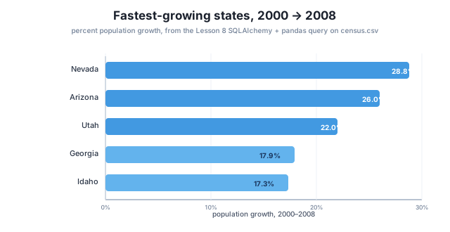
Compute each state’s percentage growth from 2000 to 2008, and sort by growth rate rather than raw size:

with engine.connect() as conn:
    stmt = select(
        census.c.state,
        func.sum(census.c.pop2000).label("pop2000"),
        func.sum(census.c.pop2008).label("pop2008"),
    ).group_by(census.c.state)
    rows = conn.execute(stmt).fetchall()

growth = [
    (row.state, row.pop2008 - row.pop2000, (row.pop2008 - row.pop2000) / row.pop2000 * 100)
    for row in rows
]
growth.sort(key=lambda item: item[2], reverse=True)

for state, change, pct in growth[:5]:
    print(state, f"{change:,}", f"{pct:.1f}%")

Output:

Nevada 577,131 28.8%
Arizona 1,336,836 26.0%
Utah 492,244 22.0%
Georgia 1,460,732 17.9%
Idaho 224,354 17.3%

This query computes the raw totals in SQL, then finishes the percentage calculation in Python — a common and perfectly reasonable split. SQL is efficient at aggregating rows; a small amount of arithmetic on the resulting 51 rows is easier to read in Python than nested inside the SQL itself.

Step 4: A Weighted Average Across Groups#

The census data has one row per age group, not one row per person — so finding the average age requires weighting each age by how many people are that age, not just averaging the age values themselves:

with engine.connect() as conn:
    stmt = select(
        census.c.sex,
        (func.sum(census.c.age * census.c.pop2000) / func.sum(census.c.pop2000)).label("avg_age"),
    ).group_by(census.c.sex)

    for row in conn.execute(stmt):
        print(row.sex, round(row.avg_age, 1))

Output:

F 37.0
M 34.5

func.sum(age * pop2000) multiplies each row’s age by its population before summing — this is the standard trick for computing a weighted average in SQL: multiply, sum, then divide by the sum of the weights. Women’s average age was almost three years higher than men’s in the 2000 data, consistent with women’s longer average life expectancy skewing the population toward older ages.

Step 5: Where Women Are the Majority#

Combine case(), cast(), and group_by() to compute what percentage of each state’s 2008 population was female:

from sqlalchemy import case, cast, Float

with engine.connect() as conn:
    stmt = select(
        census.c.state,
        (
            cast(func.sum(case((census.c.sex == "F", census.c.pop2008), else_=0)), Float)
            / cast(func.sum(census.c.pop2008), Float) * 100
        ).label("female_pct"),
    ).group_by(census.c.state)
    rows = conn.execute(stmt).fetchall()

top_female_share = sorted(rows, key=lambda row: row.female_pct, reverse=True)[:5]
for row in top_female_share:
    print(row.state, round(row.female_pct, 2))

Output:

District of Columbia 52.88
Maryland 51.76
Rhode Island 51.74
Mississippi 51.74
Delaware 51.67

Every state’s population is close to an even split, but the District of Columbia stands out — a pattern consistent with its unusually high share of older residents and federal-government employment, both of which skew toward a larger female population.

Step 6: From Query to Chart#

The final step turns your SQL result into something visual. Convert the state totals from Step 2 into a pandas DataFrame, then plot it with matplotlib:

import matplotlib.pyplot as plt

with engine.connect() as conn:
    stmt = select(census.c.state, func.sum(census.c.pop2008).label("total_pop")).group_by(census.c.state)
    rows = conn.execute(stmt).fetchall()

df = pd.DataFrame(rows, columns=["state", "total_pop"])
print(df.head(3))

top10 = df.sort_values("total_pop", ascending=False).head(10)

fig, ax = plt.subplots(figsize=(10, 6))
top10.plot(kind="bar", x="state", y="total_pop", ax=ax, legend=False, color="#4299e1")
ax.set_title("Total Population by State, 2008")
ax.set_xlabel("State")
ax.set_ylabel("Population")
plt.tight_layout()
plt.savefig("population_by_state.svg", format="svg")

Output:

     state  total_pop
0  Alabama    4649367
1   Alaska     664546
2   Arizona   6480767

pd.DataFrame(rows, columns=[...]) turns the list of result rows straight into a DataFrame — the same conversion you would use for any SQLAlchemy query result you want to hand off to pandas for plotting, exporting, or further analysis. plt.savefig(..., format="svg") writes the chart as a scalable, resolution-independent image, the same format used for the population-growth figure above.

Practice Exercises#

Extend the analysis on your own, using the same census.db database.

Exercise 1: The Ten Least-Populous States#

Adapt Step 2’s query to find the ten smallest states by 2008 population instead of the largest.

# Your code here

Exercise 2: The Five Slowest-Growing States#

Adapt Step 3’s growth calculation to find the five states with the lowest (or most negative) percentage growth from 2000 to 2008.

# Your code here

Exercise 3: Plot the Fastest-Growing States#

Build a DataFrame from Step 3’s growth data and plot the five fastest-growing states as a bar chart, similar to Step 6.

# Your code here

Summary#

You loaded a real, 8,772-row Census dataset into SQLite with pandas and a SQLAlchemy engine, then used func.sum(), group_by(), case(), and cast() — everything from this module — to find the most populous states, the fastest-growing ones, a weighted average age by sex, and each state’s female population share. Finally, you converted a query result into a pandas DataFrame and plotted it with matplotlib.

Key Concepts#

• df.to_sql(table, con=engine, if_exists="append") — loads a pandas DataFrame into a database table through a SQLAlchemy engine.
• Weighted average — SUM(value * weight) / SUM(weight), needed whenever a dataset has one row per group rather than one row per individual.
• Splitting work between SQL and Python — aggregate in SQL, finish small calculations (like a percentage across 51 rows) in Python when that is more readable.
• pd.DataFrame(rows, columns=[...]) — converts a SQLAlchemy query result directly into a DataFrame for further analysis or plotting.

Why This Matters#

This is the complete, real-world shape of a SQLAlchemy project: load real data, ask a business or research question, translate it into a query using the exact tools from this module, and visualize the answer for someone who will never read your code. Every technique here — grouping, weighted averages, conditional aggregation, and the hand-off to pandas — scales directly to a production dataset with millions of rows, running against PostgreSQL instead of SQLite, with nothing but the connection string changing.

Next Steps#

Congratulations — by finishing this lesson you have completed the entire SQL & Databases course! You started by writing your first SELECT statement and have arrived at building declarative ORM models, tuning query performance, and analyzing real Census data with SQLAlchemy and pandas. That is the full arc from querying data to building the Python programs that manage it, and it is exactly the toolkit modern data teams expect. Be proud of how far you have come.

Continue Building Your Skills#

Keep the momentum going. Apply what you learned here to a database of your own — reflect its tables, query it with Core, model it with the ORM, and see what it can tell you. If you want to go deeper into SQLAlchemy specifically, look into Alembic for schema migrations and async SQLAlchemy for high-concurrency applications. And if you want to see SQLAlchemy at work inside a real application, the FastAPI course’s Databases with SQLModel module builds directly on the same Core and ORM concepts you just learned, wired into a working API. You now have the skills to build exactly that. Well done, and keep building.