Lesson 1 - Guided Project: Build & Train Your Own Mini-GPT

Welcome to the Guided Project#

This is the last lesson of the course, and it does something none of the others could: it runs the whole transformer, end to end, as one program. Every module before this built a single part and proved it correct in isolation — attention, multiple heads, positional embeddings, the transformer block, the causal mask, the training loop, the sampling strategies. You verified each one on its own. What you have not done yet is put all eight together, point them at the Lantern Bay corpus, and watch a language model come to life from nothing but NumPy.

That is the entire project. In four stages you will assemble the mini-GPT from the components of Modules 1 through 6, train it with the Adam optimizer from Module 7, generate text from it with the decoding strategies from Module 8, and then write the final report — a trace of the finished model back through every module by name, with the concrete role each one plays and a real number to anchor it. No new theory. This lesson is the moment all the theory becomes a working thing you built yourself.

The model is deliberately tiny — n_embd=64, n_head=4, n_layer=3, block_size=32, about 154 thousand parameters — small enough that the full training run finishes in under half a minute on a laptop CPU, yet structurally identical to a real GPT. Shrink GPT-2 and you get this; grow this and you get GPT-2. Everything is seeded, so every number below reproduces exactly, and you can run each block twice to confirm it.

By the end of this project, you will be able to:

• Instantiate the complete MiniGPT from its eight-module components and read off its 154,456-parameter budget
• Confirm the forward pass produces (B, T, 24) logits and an initial loss right at log(24) = 3.18
• Run the full Adam training loop and watch train and validation loss fall from 3.20 to about 0.13 in roughly 24 seconds
• Generate text with greedy decoding and with temperature-plus-top-k sampling, and read the difference in the output
• Trace the finished model back through all eight modules, naming the role each plays in the network you just ran

This project assumes every earlier module. You only need numpy — no PyTorch, no GPU, no API key.

Stage 1: Assemble the Model (Modules 1-6)#

We begin with the corpus, the character tokenizer, and the operations the course has used throughout: a numerically stable softmax, a get_batch sampler, and the Adam optimizer you implemented in Module 7. This is the same Lantern Bay passage from every lesson — original text, 24 distinct characters, 10,020 characters long after the repetition that gives a tiny model a learnable target.

import numpy as np, time
import warnings
warnings.filterwarnings("ignore")

CORPUS = (
    "the lamp keeper walks the shore at dusk. "
    "the lamp keeper lights the lantern when the fog rolls in. "
    "the boats come home when the lantern glows. "
    "the boats wait outside the bay when the fog is thick. "
    "a small boat drifts near the rocks at dawn. "
    "the keeper rings the bell when a boat drifts near the rocks. "
    "the tide rises at dusk and falls at dawn. "
    "the gulls call over the bay when the tide is low. "
    "the keeper counts the boats and writes the count in a book. "
    "the lantern burns all night and rests at dawn. "
) * 20

chars = sorted(set(CORPUS)); vocab_size = len(chars)
stoi = {c: i for i, c in enumerate(chars)}
itos = {i: c for i, c in enumerate(chars)}
encode = lambda s: [stoi[c] for c in s]
decode = lambda ids: "".join(itos[i] for i in ids)
data = np.array(encode(CORPUS), dtype=np.int64)

def softmax(x, axis=-1):
    x = x - x.max(axis=axis, keepdims=True)      # stable: subtract row max
    e = np.exp(x)
    return e / e.sum(axis=axis, keepdims=True)

def get_batch(dat, block_size, batch_size, rng):
    ix = rng.integers(0, len(dat) - block_size - 1, size=batch_size)
    x = np.stack([dat[i:i + block_size] for i in ix])
    y = np.stack([dat[i + 1:i + block_size + 1] for i in ix])
    return x, y

class Adam:
    def __init__(self, params, lr=3e-3, b1=0.9, b2=0.999, eps=1e-8):
        self.lr, self.b1, self.b2, self.eps = lr, b1, b2, eps; self.t = 0
        self.m = {k: np.zeros_like(v) for k, v in params.items()}
        self.v = {k: np.zeros_like(v) for k, v in params.items()}
    def step(self, params, grads):
        self.t += 1
        for k in params:
            g = grads[k]
            self.m[k] = self.b1 * self.m[k] + (1 - self.b1) * g
            self.v[k] = self.b2 * self.v[k] + (1 - self.b2) * (g * g)
            mh = self.m[k] / (1 - self.b1 ** self.t)
            vh = self.v[k] / (1 - self.b2 ** self.t)
            params[k] -= self.lr * mh / (np.sqrt(vh) + self.eps)

Now the model itself. Rather than carry a separate TransformerBlock object, the capstone keeps every weight in one flat dictionary self.P and runs the whole forward and backward inline — the same math you derived module by module, gathered into two methods. Read the __init__ as a parts list: the token embedding E and position table P are Module 4; each layer’s Wq, Wk, Wv, Wo are the multi-head attention of Modules 2 and 3; the two LayerNorms and the W1/W2 feed-forward network are the transformer block of Module 5; and the final norm plus the head Wh/bh are the language-modeling head of Module 6. The causal mask that makes it a GPT lives in forward.

class MiniGPT:
    def __init__(self, vocab_size, block_size, n_embd, n_head, n_layer, seed=42):
        rng = np.random.default_rng(seed)
        self.cfg = (vocab_size, block_size, n_embd, n_head, n_layer)
        self.n_head, self.n_layer, self.hs = n_head, n_layer, n_embd // n_head
        P = {}; s = 0.02
        P['E'] = rng.normal(0, s, (vocab_size, n_embd))       # token embedding  (Module 4)
        P['P'] = rng.normal(0, s, (block_size, n_embd))       # position table   (Module 4)
        for l in range(n_layer):                              # transformer block (Module 5)
            P[f'ln1g{l}'] = np.ones(n_embd); P[f'ln1b{l}'] = np.zeros(n_embd)
            P[f'Wq{l}'] = rng.normal(0, s, (n_embd, n_embd))  # query/key/value  (Modules 2-3)
            P[f'Wk{l}'] = rng.normal(0, s, (n_embd, n_embd))
            P[f'Wv{l}'] = rng.normal(0, s, (n_embd, n_embd))
            P[f'Wo{l}'] = rng.normal(0, s, (n_embd, n_embd))  # output projection (Module 3)
            P[f'ln2g{l}'] = np.ones(n_embd); P[f'ln2b{l}'] = np.zeros(n_embd)
            P[f'W1{l}'] = rng.normal(0, s, (n_embd, 4 * n_embd)); P[f'b1{l}'] = np.zeros(4 * n_embd)
            P[f'W2{l}'] = rng.normal(0, s, (4 * n_embd, n_embd)); P[f'b2{l}'] = np.zeros(n_embd)
        P['lnfg'] = np.ones(n_embd); P['lnfb'] = np.zeros(n_embd)
        P['Wh'] = rng.normal(0, s, (n_embd, vocab_size))      # LM head          (Module 6)
        P['bh'] = np.zeros(vocab_size)
        self.P = P
    def n_params(self): return sum(v.size for v in self.P.values())

    def _ln_f(self, x, g, b):
        mu = x.mean(-1, keepdims=True); xc = x - mu
        var = (xc ** 2).mean(-1, keepdims=True); std = np.sqrt(var + 1e-5)
        xh = xc / std; return g * xh + b, (xh, std, g)

    def _ln_b(self, dout, cache):
        xh, std, g = cache; C = xh.shape[-1]; dxh = dout * g
        dx = (1 / (C * std)) * (C * dxh - dxh.sum(-1, keepdims=True)
                                - xh * (dxh * xh).sum(-1, keepdims=True))
        return dx, (dout * xh).reshape(-1, C).sum(0), dout.reshape(-1, C).sum(0)

    def forward(self, idx, targets=None):
        V, BS, C, H, L = self.cfg; B, T = idx.shape; P = self.P; hs = self.hs; ca = {}
        x = P['E'][idx] + P['P'][:T]; ca['idx'] = idx; ca['T'] = T          # embed + position (Module 4)
        mask = np.triu(np.ones((T, T), dtype=bool), k=1)                     # causal mask (Module 6)
        for l in range(L):                                                   # transformer blocks (Module 5)
            ln1, c1 = self._ln_f(x, P[f'ln1g{l}'], P[f'ln1b{l}'])
            Q = (ln1 @ P[f'Wq{l}']).reshape(B, T, H, hs).transpose(0, 2, 1, 3)   # multi-head (Modules 2-3)
            K = (ln1 @ P[f'Wk{l}']).reshape(B, T, H, hs).transpose(0, 2, 1, 3)
            Vv = (ln1 @ P[f'Wv{l}']).reshape(B, T, H, hs).transpose(0, 2, 1, 3)
            sc = Q @ K.transpose(0, 1, 3, 2) / np.sqrt(hs)                       # scaled dot product (Module 2)
            sc = np.where(mask, -1e9, sc); A = softmax(sc, -1)                   # mask then softmax
            ho = (A @ Vv).transpose(0, 2, 1, 3).reshape(B, T, C); att = ho @ P[f'Wo{l}']
            x2 = x + att                                                          # residual 1 (Module 5)
            ln2, c2 = self._ln_f(x2, P[f'ln2g{l}'], P[f'ln2b{l}'])
            h = ln2 @ P[f'W1{l}'] + P[f'b1{l}']; hr = np.maximum(h, 0)            # feed-forward (Module 5)
            ff = hr @ P[f'W2{l}'] + P[f'b2{l}']
            x = x2 + ff                                                           # residual 2 (Module 5)
            ca[l] = (ln1, c1, Q, K, Vv, A, ho, x2, ln2, c2, h, hr)
        xf, cf = self._ln_f(x, P['lnfg'], P['lnfb']); logits = xf @ P['Wh'] + P['bh']   # LM head (Module 6)
        ca['xf'] = xf; ca['cf'] = cf; self.ca = ca
        if targets is None: return logits, None
        B, T, Vt = logits.shape; flat = logits.reshape(-1, Vt); tgt = targets.reshape(-1)
        p = softmax(flat, -1); loss = -np.log(p[np.arange(len(tgt)), tgt] + 1e-12).mean()   # cross-entropy (Module 6)
        self.ca['p'] = p; self.ca['tgt'] = tgt; self.ca['shape'] = (B, T, Vt)
        return logits, loss

    def backward(self):
        V, BS, C, H, L = self.cfg; P = self.P; hs = self.hs; ca = self.ca
        g = {k: np.zeros_like(v) for k, v in P.items()}
        p = ca['p'].copy(); tgt = ca['tgt']; B, T, Vt = ca['shape']; N = len(tgt)
        p[np.arange(N), tgt] -= 1; dlogits = (p / N).reshape(B, T, Vt)       # (probs - onehot) / N
        xf = ca['xf']
        g['Wh'] = xf.reshape(-1, C).T @ dlogits.reshape(-1, Vt); g['bh'] = dlogits.reshape(-1, Vt).sum(0)
        dxf = dlogits @ P['Wh'].T
        dx, g['lnfg'], g['lnfb'] = self._ln_b(dxf, ca['cf'])
        mask = np.triu(np.ones((T, T), dtype=bool), k=1)
        for l in reversed(range(L)):
            ln1, c1, Q, K, Vv, A, ho, x2, ln2, c2, h, hr = ca[l]
            dx2 = dx.copy(); dff = dx                                        # residual 2 splits the gradient
            g[f'W2{l}'] = hr.reshape(-1, 4 * C).T @ dff.reshape(-1, C); g[f'b2{l}'] = dff.reshape(-1, C).sum(0)
            dhr = dff @ P[f'W2{l}'].T; dh = dhr * (h > 0)
            g[f'W1{l}'] = ln2.reshape(-1, C).T @ dh.reshape(-1, 4 * C); g[f'b1{l}'] = dh.reshape(-1, 4 * C).sum(0)
            dln2 = dh @ P[f'W1{l}'].T
            dx2b, g[f'ln2g{l}'], g[f'ln2b{l}'] = self._ln_b(dln2, c2); dx2 = dx2 + dx2b
            dx1 = dx2.copy(); datt = dx2                                     # residual 1 splits the gradient
            g[f'Wo{l}'] = ho.reshape(-1, C).T @ datt.reshape(-1, C)
            dho = datt @ P[f'Wo{l}'].T
            dHe = dho.reshape(B, T, H, hs).transpose(0, 2, 1, 3)
            dA = dHe @ Vv.transpose(0, 1, 3, 2); dValue = A.transpose(0, 1, 3, 2) @ dHe
            dsc = A * (dA - (dA * A).sum(-1, keepdims=True)); dsc = np.where(mask, 0, dsc) / np.sqrt(hs)
            dQuery = dsc @ K; dKey = dsc.transpose(0, 1, 3, 2) @ Q           # gradients of Q, K, V
            def merge(t): return t.transpose(0, 2, 1, 3).reshape(B, T, C)
            dQm, dKm, dVm = merge(dQuery), merge(dKey), merge(dValue)
            g[f'Wq{l}'] = ln1.reshape(-1, C).T @ dQm.reshape(-1, C)
            g[f'Wk{l}'] = ln1.reshape(-1, C).T @ dKm.reshape(-1, C)
            g[f'Wv{l}'] = ln1.reshape(-1, C).T @ dVm.reshape(-1, C)
            dln1 = dQm @ P[f'Wq{l}'].T + dKm @ P[f'Wk{l}'].T + dVm @ P[f'Wv{l}'].T
            dx1b, g[f'ln1g{l}'], g[f'ln1b{l}'] = self._ln_b(dln1, c1); dx1 = dx1 + dx1b
            dx = dx1
        np.add.at(g['E'], ca['idx'], dx); g['P'][:T] = dx.sum(axis=0)        # scatter-add into E; sum into P
        return g

That is the whole model in one class. Note the naming inside backward: the gradients of the query, key, and value are dQuery, dKey, and dValue — the convention we have used since Module 2, keeping the forward variables Q, K, V and giving their gradients readable names. Now instantiate the model at the course’s canonical config and run one forward pass to sanity-check the shapes and the initial loss.

block_size, n_embd, n_head, n_layer = 32, 64, 4, 3
model = MiniGPT(vocab_size, block_size, n_embd, n_head, n_layer, seed=42)
print("vocab_size:", vocab_size, "| corpus length:", len(data))
print("config: block_size=%d n_embd=%d n_head=%d n_layer=%d head_size=%d"
      % (block_size, n_embd, n_head, n_layer, model.hs))
print("parameters:", model.n_params())

rng0 = np.random.default_rng(42)
xb, yb = get_batch(data, block_size, 32, rng0)
logits, loss = model.forward(xb, yb)
print("input idx :", xb.shape)
print("logits    :", logits.shape)
print("init loss :", round(float(loss), 4), "| log(24) =", round(float(np.log(24)), 4))

vocab_size: 24 | corpus length: 10020
config: block_size=32 n_embd=64 n_head=4 n_layer=3 head_size=16
parameters: 154456
input idx : (32, 32)
logits    : (32, 32, 24)
init loss : 3.2011 | log(24) = 3.1781

Three numbers confirm the assembly is correct. The model has 154,456 parameters — small by any modern standard, large enough to learn this corpus. The logits come out (32, 32, 24): for each of the 32 sequences and each of the 32 positions, a full distribution over the 24 characters. And the initial loss is 3.2011, right next to log(24) = 3.1781 — the fingerprint of a fresh language model that has no idea what comes next and spreads its probability almost uniformly over all 24 characters. Everything is wired; nothing is trained.

Stage 2: Train the Model (Module 7)#

The model is assembled and its forward and backward passes were gradient-checked back in Module 6. Training is now nothing more than the loop from Module 7: sample a batch, run forward to get the loss, run backward to get the gradients, and let Adam nudge every parameter. We split the corpus 90/10 into train and validation so we can watch both, sample the loss every 100 steps, and run 1200 steps total. Everything is seeded, so the loss curve below is exact.

model = MiniGPT(vocab_size, block_size, n_embd, n_head, n_layer, seed=42)
opt = Adam(model.P, lr=3e-3)

n = int(len(data) * 0.9); train_data, val_data = data[:n], data[n:]
rng = np.random.default_rng(42)

t0 = time.time()
for step in range(1201):
    xb, yb = get_batch(train_data, block_size, 32, rng)
    _, loss = model.forward(xb, yb)
    grads = model.backward()
    opt.step(model.P, grads)
    if step % 100 == 0:
        xv, yv = get_batch(val_data, block_size, 32, rng)
        _, vloss = model.forward(xv, yv)
        print(f"step {step:4d}  train {loss:.4f}  val {vloss:.4f}")
wall = time.time() - t0
print(f"final train loss {loss:.4f}  |  wall-clock {wall:.1f}s")

step    0  train 3.2026  val 2.9061
step  100  train 0.4645  val 0.4260
step  200  train 0.2056  val 0.1723
step  300  train 0.1577  val 0.1339
step  400  train 0.1432  val 0.1436
step  500  train 0.1544  val 0.1362
step  600  train 0.1634  val 0.1440
step  700  train 0.1257  val 0.1254
step  800  train 0.1440  val 0.1365
step  900  train 0.1271  val 0.1336
step 1000  train 0.2204  val 0.1651
step 1100  train 0.1330  val 0.1405
step 1200  train 0.1337  val 0.1362

final train loss 0.1337  |  wall-clock 23.9s

There it is: a transformer training itself in pure NumPy in about 24 seconds. The loss starts at 3.2026 — the uniform-guess baseline — and by step 100 it has already collapsed to 0.46, because the easiest patterns (spaces follow words, t is usually followed by h, the is everywhere) are learned almost immediately. From there it grinds down to around 0.13 and hovers, the model now confidently predicting each next character from its context. Notice that train and validation track each other closely the whole way — around 0.13 each at the end — which tells us the model is genuinely learning the structure of the text, not just memorizing individual training windows. On a corpus this small and repetitive that is exactly what we want to see.

Stage 3: Generate Text (Module 8)#

A trained model does not produce text — it produces, at each step, a distribution over the next character. Turning that into a sequence is the decoding problem from Module 8. We generate autoregressively: feed the current context (clipped to the last block_size characters), take the model’s last-position logits, choose a next character, append it, and repeat. The only thing that changes between strategies is how we choose.

def generate(model, prompt, n_new, rng, temperature=1.0, top_k=None, greedy=False):
    ids = encode(prompt); BS = model.cfg[1]
    for _ in range(n_new):
        ctx = np.array([ids[-BS:]])                 # last block_size chars
        logits, _ = model.forward(ctx)
        row = logits[0, -1] / temperature           # next-char logits
        if greedy:
            nxt = int(row.argmax())                 # always the most likely char
        else:
            if top_k is not None:                   # keep only the top-k logits
                thresh = np.sort(row)[-top_k]
                row = np.where(row < thresh, -1e9, row)
            probs = softmax(row)
            nxt = int(rng.choice(len(probs), p=probs))
        ids.append(nxt)
    return decode(ids)

g_greedy = generate(model, "the ", 80, rng, greedy=True)
print("GREEDY           :", repr(g_greedy))

rng_s = np.random.default_rng(7)
g_sample = generate(model, "the ", 80, rng_s, temperature=0.8, top_k=10)
print("TEMP=0.8 TOP_K=10:", repr(g_sample))

GREEDY           : 'the boats and writes the count in a booat ide rise the bay when the fog is thick. a '
TEMP=0.8 TOP_K=10: 'the lantern glows. the boats wait outside the bay when the fog is thick. a small boa'

This is a language model you built from scratch writing English. Greedy decoding — always taking the single most likely next character — produces mostly coherent Lantern Bay text (the boats ... writes the count in a boo..., the bay when the fog is thick), but you can see its known failure mode: it slips at booat ide rise, because always taking the top character can wander into a locally-likely but globally-wrong groove and get briefly stuck. Temperature-plus-top-k sampling — soften the distribution with temperature=0.8, keep only the 10 most likely characters, and sample — reads more smoothly here: the lantern glows. the boats wait outside the bay when the fog is thick. a small boa.... It draws whole clean sentences straight from the corpus’s structure while retaining the freedom to pick a different continuation each run.

Because sampling draws from a random generator, its output depends on the seed: greedy is deterministic and reproduces exactly every time, while the sampled text changes if you pass a different rng. That is the point of sampling — variety — and swapping the seed is how you get a different valid continuation from the same trained model.

The Final Report#

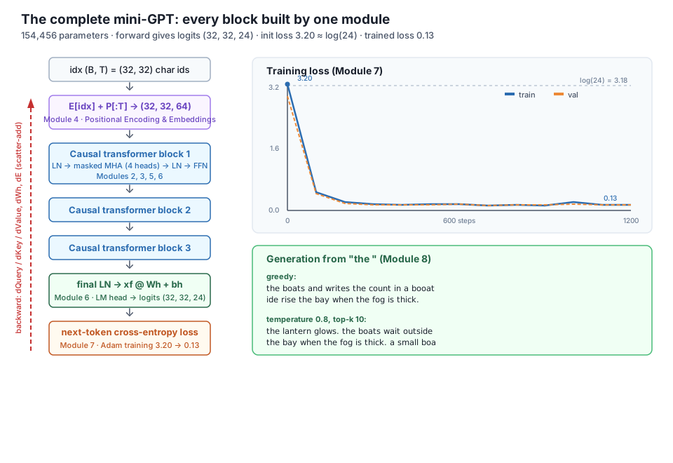
You have run the whole thing. Here is the finished model traced back through all eight modules, each with the concrete role it plays in the network you just trained and a real number to anchor it.

Module 1 — From Sequences to Attention. This module made the case for the entire architecture: that a recurrent network’s fixed-size hidden state is a bottleneck, and that attention — a content-based weighted lookup where every position pulls from every other — is the fix. That idea is the load-bearing operation of your model. Each of the 3 layers runs it, and the A = softmax(sc, -1) matrix in forward is exactly the “soft lookup table” Module 1 introduced, now computed for real over the Lantern Bay corpus.

Module 2 — Self-Attention from Scratch. This gave you the precise mechanism: the query, key, and value projections and scaled dot-product attention, sc = Q @ K.transpose(...) / np.sqrt(hs). The 1/√hs scaling — with hs = 16 here, so a divisor of 4 — is the line that keeps the scores from saturating the softmax, and Module 2 is where you proved by hand that the backward pass through it is correct. That derivation is the dsc, dQuery, dKey, dValue block inside backward.

Module 3 — Multi-Head Attention. One head sees one relationship; your model runs n_head = 4 in parallel, each of size 16. The .reshape(B, T, H, hs).transpose(0, 2, 1, 3) split, the parallel attention, the concatenation back to width 64, and the output projection Wo are all straight from this module. Four heads per layer, three layers — twelve attention heads working at once every forward pass.

Module 4 — Positional Encoding & Embeddings. Attention is permutation-invariant, so this module gave the model a sense of order. The very first line of forward, x = P['E'][idx] + P['P'][:T], is its product: the token embedding E (24 x 64) says what each character is, and the learned position table P (32 x 64) says where it sits. Without that P, the model could not tell "the boat" from "boat the".

Module 5 — The Transformer Block. This module built everything around attention that makes a deep stack trainable: the two residual connections (x2 = x + att, x = x2 + ff), the LayerNorm before each sublayer, and the position-wise feed-forward network that expands 64 to 256 and back. Your model stacks this block 3 times. The residuals are why the gradient survives all three layers; the LayerNorm is why the activations stay well-scaled; the feed-forward network is where most of the 154,456 parameters actually live.

Module 6 — Causal Masking & GPT. This turned the stack into a GPT. The mask = np.triu(...) and sc = np.where(mask, -1e9, sc) lines forbid a position from attending to the future, so that predicting the next character from the past is a fair task. This module also added the language-modeling head (Wh, bh) projecting each position to 24 logits and the next-token cross-entropy loss — the 3.2011 you saw on the first forward pass.

Module 7 — Training a Tiny GPT. This module supplied the machinery that made the loss move: the get_batch sampler, the Adam optimizer you implemented from its running averages and bias correction, and the forward-loss-backward-update loop. Running it for 1200 steps drove the loss from 3.2026 to 0.1337 in about 24 seconds, with train and validation tracking together near 0.13 — the difference between a random model and a trained one.

Module 8 — Generation & Sampling. Finally, this module turned the trained distribution into text. The greedy decoder and the temperature-plus-top-k sampler in generate are its contribution: greedy gave you 'the boats and writes the count in a boo...', and temperature=0.8, top_k=10 gave you 'the lantern glows. the boats wait outside the bay...'. Same model, two decoding strategies, two different-feeling outputs — the last choice in the pipeline.

Eight modules, one working language model, every line of it yours.

Practice Exercises#

These are reflective — they ask you to reason about the whole model you built, then confirm your reasoning by running a small change.

Exercise 1: Predict, then measure, the effect of temperature#

Before running anything, predict what temperature=0.5 versus temperature=1.5 will do to the generated text, thinking back to Module 8. Then generate 80 characters from "the " at each temperature (keep top_k=10, use a fresh seeded rng for each) and compare. Which one reads more like clean corpus text, and which one takes more risks? Does the result match your prediction?

Exercise 2: Locate where the parameters actually live#

The model has 154,456 parameters. Reason about which component holds the most — the embeddings, the attention projections, or the feed-forward networks — then confirm it by summing the sizes in model.P grouped by name. Does the answer square with what Module 5 said about the feed-forward network being the widest part of the block?

Exercise 3: Break one module and watch the model fail#

Pick a single module’s contribution and disable it to see how much the model depends on it. The cleanest experiment is Module 4’s position table: retrain a fresh model with P['P'] forced to zeros (so the model gets no position signal), and compare the final loss and generated text to the real run. What does the loss floor become, and why can a model with no sense of order not learn this corpus as well?

Summary#

You assembled, trained, and sampled from a complete transformer — the entire course, running end to end in pure NumPy.

Key Concepts#

Assembly (Modules 1-6)

• One MiniGPT class holds every weight in a flat dict self.P: token embedding E and position table P (Module 4), per-layer Wq/Wk/Wv/Wo multi-head attention (Modules 2-3), LayerNorms and the W1/W2 feed-forward network (Module 5), and the final norm plus Wh/bh head (Module 6)
• At n_embd=64, n_head=4, n_layer=3, block_size=32 the model has 154,456 parameters; the forward pass returns (32, 32, 24) logits and an initial loss of 3.2011, right at log(24) = 3.178
• The backward pass names the query/key/value gradients dQuery, dKey, dValue and finishes with a scatter-add into E

Training (Module 7)

• The loop is forward, loss, backward, Adam.step, repeated 1200 times; train and validation loss both fall from about 3.20 to about 0.13 in roughly 24 seconds
• The loss floors near 0.13 rather than zero because the corpus has real next-character ambiguity — the irreducible entropy — and train and validation tracking together shows genuine learning, not memorization

Generation (Module 8)

• Greedy decoding is deterministic and mostly coherent but can get briefly stuck; temperature-plus-top-k sampling (temperature=0.8, top_k=10) reads more smoothly and varies with the seed
• Both run on the same trained logits — decoding is a choice made after training, not part of it

Why This Matters#

Everything in a modern large language model is in the code you just ran. GPT-2, GPT-3, and the models behind today’s assistants are this exact object — token and position embeddings, a stack of causal multi-head-attention blocks with residuals and layer norm and feed-forward networks, a language-modeling head, next-token cross-entropy loss, an Adam optimizer, and a decoding strategy — scaled up by a few orders of magnitude in width, depth, data, and compute, with engineering refinements layered on top. Not one of those systems contains a component you have not now built and verified by hand.

That is the real payoff of doing it from scratch. When you read that a frontier model has a context window, you know that is block_size. When you read that it was trained on next-token prediction, you know that is the cross-entropy loss you watched fall from 3.20. When you hear about temperature or top-k in an API, you know exactly which line of generate that is. The vocabulary of the field is no longer jargon — it is a set of arrays and operations you can point to in your own 154,456-parameter model. You did not learn about transformers; you built one.

Continue Building Your Skills#

You have reached the end of the course with a complete, working, from-scratch transformer that you understand line by line — and that is a rare foundation. The natural next step is to make this model bigger and see how far the same code carries: raise n_layer to six or eight, widen n_embd, lengthen block_size, and feed it a larger original corpus, watching the loss floor drop as capacity and data grow. Everything you built scales without new ideas, which is precisely the lesson the last decade of the field has taught. From here you might explore the refinements that separate a toy from a production model — a proper byte-pair tokenizer instead of characters, dropout and weight decay for regularization, learning-rate warmup and decay, and the KV-caching trick that makes generation fast — each of which is a small, understandable addition to the machinery you already own. But whatever you build next, you now carry the thing that matters most: you know what is actually happening inside a transformer, because you wrote every operation yourself.