Title here
Summary here
You have built every mechanical part of a transformer: token and position embeddings, scaled dot-product attention, multi-head attention, and the full transformer block with residuals and layer norm. What you do not yet have is a reason for the model to compute anything, an objective that turns a stack of matrix multiplies into something that learns language. This module supplies that objective, and it is astonishingly simple: predict the next token.
That single idea, done at every position of a sequence and repeated over a corpus, is all that GPT is trained to do. In this first lesson you will not build any new model machinery. Instead you will set up the learning problem the rest of the module solves: how a language model assigns probability to text, how you turn a raw token sequence into supervised (input, target) pairs by shifting it, and why a transformer can make all of a sequence’s next-token predictions at once, in parallel, where a recurrent network has to crawl through them one step at a time. You will finish by computing the score a completely untrained model achieves, the baseline your GPT has to beat.
By the end of this lesson, you will be able to:
inputs = tokens[:-1] and targets = tokens[1:], and verify targets[t] == inputs[t+1]You should already be comfortable with the char-level tokenization from Module 3 and the (B, T, C) activation convention we use everywhere. Let’s begin.
Suppose you want a model to assign a probability to a whole sequence of characters, say the string the lantern. That looks like a hard joint-probability problem: there are possible strings of length over a vocabulary of size , and no model can store a number for each one. The autoregressive trick sidesteps this entirely by using the chain rule of probability to break the joint into a product of one-step conditionals:
Read left to right, this says: the probability of the whole sequence is the probability of the first token, times the probability of the second given the first, times the probability of the third given the first two, and so on. Each factor is a distribution over the vocabulary, conditioned on everything that came before position . That is exactly what our model will output at each position: a length- vector of probabilities for “what comes next.”
Nothing here is approximate. The factorization above is an exact identity, true for any joint distribution. What makes it useful is that it reduces one impossible -way problem to copies of the same manageable problem: given a context, produce a distribution over the next single token. A language model is nothing more than a function that answers that one question, reused at every position.
Training the model means adjusting its weights so that the probability it assigns to the actual next token, the one that really followed in the corpus, is as high as possible, at every position of every training sequence. Equivalently, we minimize the negative log of that probability, averaged over positions. That average negative log-probability is the cross-entropy loss, and it is the number that will drop as the model learns. We derive its gradient in Lesson 4; for now the important thing is the shape of the problem: a supervised prediction at every position, with the true next token as the label.
Why the log turns a product into a sum
Maximizing the product directly is numerically miserable: multiplying thousands of numbers below 1 underflows to zero. Taking the logarithm converts the product into a sum, , which is stable to compute and, conveniently, has a per-position gradient. Minimizing the negative log-probability per token is precisely the cross-entropy loss you will implement later in this module.
To make everything concrete we use the course’s canonical corpus, the tiny original passage about the town of Lantern Bay, tokenized at the character level exactly as in Module 3. The repetition (* 20) gives a small model a low-entropy, learnable target so a short training run shows the loss falling clearly later in the module.
import numpy as np

CORPUS = (
    "the lamp keeper walks the shore at dusk. "
    "the lamp keeper lights the lantern when the fog rolls in. "
    "the boats come home when the lantern glows. "
    "the boats wait outside the bay when the fog is thick. "
    "a small boat drifts near the rocks at dawn. "
    "the keeper rings the bell when a boat drifts near the rocks. "
    "the tide rises at dusk and falls at dawn. "
    "the gulls call over the bay when the tide is low. "
    "the keeper counts the boats and writes the count in a book. "
    "the lantern burns all night and rests at dawn. "
) * 20

chars = sorted(set(CORPUS))
vocab_size = len(chars)
stoi = {c: i for i, c in enumerate(chars)}
itos = {i: c for i, c in enumerate(chars)}
encode = lambda s: [stoi[c] for c in s]
decode = lambda ids: "".join(itos[i] for i in ids)
data = np.array(encode(CORPUS), dtype=np.int64)

print("vocab_size:", vocab_size)
print("len(data):", len(data))
print("chars:", repr("".join(chars)))
vocab_size: 24
len(data): 10020
chars: ' .abcdefghiklmnoprstuvwy'The vocabulary is exactly 24 symbols: the lowercase letters that appear, plus a space and a period. Every character in the corpus becomes one integer id, and the whole corpus is a flat array data of 10020 token ids. That flat array is the raw material; the next step is to carve supervised examples out of it.
Here is the entire data-labeling recipe for a language model, and it is almost too simple to believe: the target is the input shifted left by one. If the model sees the token at position , the correct answer is the token at position , the one that actually came next. So given any contiguous slice of data, we form:
inputs = tokens[:-1] — every token except the lasttargets = tokens[1:] — every token except the firstEvery input token is paired with the token that follows it. Let’s take a short slice so the pairs fit in a readable table. We use a block of length , which needs tokens (you need one extra token so the last input position has a target).
np.random.seed(42)
block_size = 12                       # context length T for this demo
chunk = data[:block_size + 1]         # need T+1 tokens to form T pairs
inputs = chunk[:-1]                   # tokens[:-1]
targets = chunk[1:]                   # tokens[1:]

print("chunk (T+1 tokens):", chunk.tolist())
print("inputs  decodes to:", repr(decode(inputs)))
print("targets decodes to:", repr(decode(targets)))
print("inputs  shape:", inputs.shape)
print("targets shape:", targets.shape)
chunk (T+1 tokens): [19, 9, 6, 0, 12, 2, 13, 16, 0, 11, 6, 6, 16]
inputs decodes to: 'the lamp kee'
targets decodes to: 'he lamp keep'
inputs shape: (12,)
targets shape: (12,)The two strings are the same text offset by one character: inputs is the lamp kee and targets is he lamp keep. That offset is the supervision. Let’s print the pairing position by position so there is no doubt about what the model is being asked to learn.
print("pos | input id | input char | target id | target char")
for t in range(block_size):
    print(f"{t:3d} | {inputs[t]:8d} | {itos[inputs[t]]!r:>10} | "
          f"{targets[t]:9d} | {itos[targets[t]]!r:>11}")
pos | input id | input char | target id | target char
0 | 19 | 't' | 9 | 'h'
1 | 9 | 'h' | 6 | 'e'
2 | 6 | 'e' | 0 | ' '
3 | 0 | ' ' | 12 | 'l'
4 | 12 | 'l' | 2 | 'a'
5 | 2 | 'a' | 13 | 'm'
6 | 13 | 'm' | 16 | 'p'
7 | 16 | 'p' | 0 | ' '
8 | 0 | ' ' | 11 | 'k'
9 | 11 | 'k' | 6 | 'e'
10 | 6 | 'e' | 6 | 'e'
11 | 6 | 'e' | 16 | 'p'Every row is one training example: “given this input character (in the context of everything to its left), predict this target character.” At position 0 the model sees t and must predict h; at position 3 it sees a space (after the) and must predict l; at position 6 it sees m and must predict p. Twelve input positions produce twelve labeled predictions from a single thirteen-token slice.
Because the target is a pure shift of the input, there is an identity that must hold: the target at position is literally the input at position . Let’s assert it in code rather than trust our eyes.
print("targets[t] == inputs[t+1] for all valid t?",
      bool(np.all(targets[:-1] == inputs[1:])))
targets[t] == inputs[t+1] for all valid t? TrueThat True confirms the shift is exactly right. It is worth internalizing this check, because an off-by-one error here, targets shifted by two, or not shifted at all, is one of the most common and most silent bugs in a language-model pipeline: the code runs, the loss even goes down, but the model is learning the wrong task.
One slice, one label array, no separate targets file
Notice we never wrote down labels by hand. The corpus is its own supervision: shift it by one and you have generated a target for every position for free. This is why language modeling is called self-supervised, and it is the reason GPT-style models can train on raw text at enormous scale, no human annotation required, only tokens[:-1] and tokens[1:].
Here is the property that makes transformers the architecture of choice for this objective. Look again at the twelve rows above. Each is an independent supervised prediction, position predicting token from the context . A recurrent network computes these one at a time: it reads token 0, updates a hidden state, emits a prediction, reads token 1, updates the state, emits the next prediction, and so on. To score a length- sequence it must take sequential steps, each waiting on the one before, because the hidden state at step depends on the hidden state at step .
A transformer does not have that dependency. With the causal mask you will build in Lesson 2, a single forward pass over the whole row produces a next-token distribution at every position simultaneously. Position is allowed to attend to positions through (its own context) but is forbidden from peeking at positions and beyond (its answer, and the future). Because the positions do not depend on each other sequentially, they are computed in parallel as one big batch of matrix multiplies. One row of length yields supervised predictions in one pass.
We do not have the model built yet, so let’s just make the shapes of that idea concrete. We reshape the single slice into a batch of one row, (B, T), which is exactly the shape a transformer consumes, and count how many predictions it implies.
B = 1
X = inputs.reshape(B, block_size)     # (B, T) — what the model reads
Y = targets.reshape(B, block_size)    # (B, T) — the label at each position

print("X (inputs)  shape:", X.shape)
print("Y (targets) shape:", Y.shape)
print("next-token predictions scored from this one row:", B * block_size)
X (inputs) shape: (1, 12)
Y (targets) shape: (1, 12)
next-token predictions scored from this one row: 12One input row of shape (1, 12) carries twelve labels and, once the model exists, will produce twelve next-token distributions in a single forward pass. Stack many such rows into a batch of shape (B, T) and you score B * T predictions at once. This parallelism over positions, made safe by the causal mask so no position cheats by reading its own answer, is the central efficiency of training a GPT, and the whole reason Lesson 2 exists.
Parallel to train, sequential to generate
The parallelism is a training advantage: at training time you already know the whole sequence, so you can score every position at once. When you generate new text (Module 8) the model is still autoregressive, it must produce one token, append it to the context, and run again, because token genuinely does not exist yet. Training in parallel, sampling step by step: both flow from the same next-token factorization.
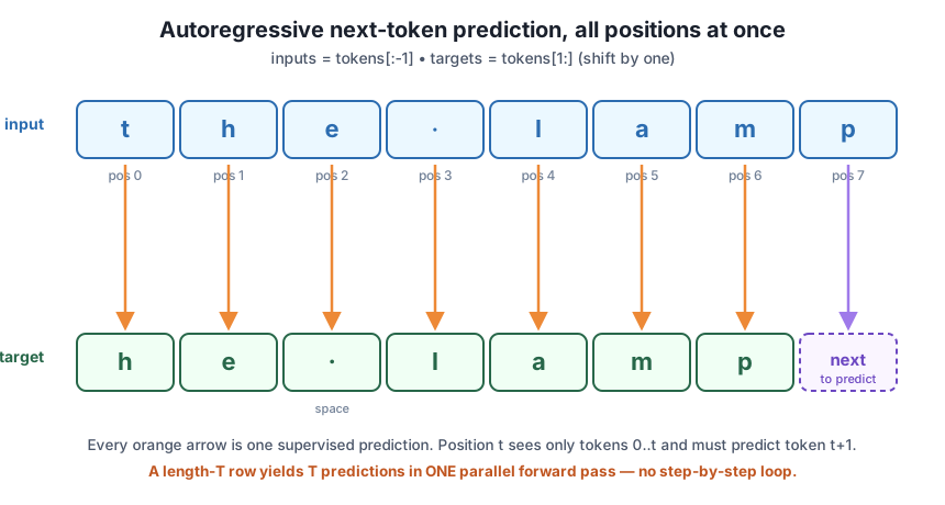
inputs = tokens[:-1]; the bottom row is targets = tokens[1:], the same text moved one step left. Each orange arrow is a single supervised next-token prediction: position t reads tokens 0..t and must output token t+1. A causal transformer computes all of these arrows in one parallel forward pass, unlike an RNN that walks them one step at a time.Before training anything, it is worth knowing what “learning nothing” scores, so you can recognize progress. Consider the dumbest possible language model: one that ignores the context entirely and predicts every one of the 24 characters with equal probability . What loss does it get?
The per-token cross-entropy loss is the negative log-probability the model assigns to the true next token. For the uniform model, whatever the true token is, it received probability , so the loss at every position is the same:
Let’s compute it, in the natural-log units (nats) our loss will use, and also convert to bits for intuition.
uniform_loss = -np.log(1.0 / vocab_size)   # = log(24)
print("uniform baseline loss (nats): -log(1/%d) = %.6f" % (vocab_size, uniform_loss))
print("uniform baseline loss (bits):            %.6f" % (uniform_loss / np.log(2)))
uniform baseline loss (nats): -log(1/24) = 3.178054
uniform baseline loss (bits): 4.584963So a model that has learned absolutely nothing about Lantern Bay scores about 3.178 nats per token (equivalently bits, which just says “it takes about 4.6 bits to name one of 24 equally likely characters”). This is the number to beat. When you train the mini-GPT in Module 7 and watch the loss print, the first thing you will check is that it starts near this value, a freshly initialized model with tiny random weights predicts almost uniformly, and then falls well below it. Because the corpus is so repetitive, a working model should eventually reach a loss far under 3.178, having learned that t is very often followed by h, that the recurs constantly, and so on.
A quick sanity anchor for later: this is the exact analogue of the “loss near ” check you used for binary classification in the Deep Learning Foundations module. There the untrained baseline was for two classes; here it is for twenty-four. Same reasoning, more classes.
Try these before checking the hints. They reuse CORPUS, data, encode, decode, itos, and vocab_size from above.
Instead of the first 13 tokens, build inputs and targets from the slice data[100:100 + block_size + 1] with block_size = 8. Print the decoded input and target strings and assert that targets[t] == inputs[t+1] still holds.
# Your code here (block_size = 8, start at index 100)Hint
Set block_size = 8, take chunk = data[100:100 + block_size + 1] (that is 9 tokens), then inputs = chunk[:-1] and targets = chunk[1:]. Use decode(inputs) and decode(targets) to see the two shifted strings, and bool(np.all(targets[:-1] == inputs[1:])) should print True. The shift identity holds for any slice, that is the whole point.
A real training step uses a batch of many rows, not one. If you stack B = 32 rows each of length T = block_size = 12 into an array of shape (B, T), how many supervised next-token predictions does one forward pass score? Compute it in code and print the shape and the count.
# Your code here: B = 32, T = 12Hint
Every position of every row is one prediction, so the count is B * T. With B = 32 and T = 12 that is 32 * 12 = 384 predictions from a single (32, 12) forward pass. This is why batching plus position-parallelism makes transformer training so throughput-efficient, hundreds of labels scored per pass, none of them waiting on a previous step.
The uniform baseline depends only on the vocabulary size. Suppose you switched from character tokens to a word-level vocabulary of V = 5000 tokens. Compute the uniform-random loss in nats and confirm it is much larger than the 3.178 you got for 24 characters. Explain in a comment why a bigger vocabulary raises the baseline.
# Your code here: V = 5000Hint
Compute -np.log(1.0 / 5000), which is log(5000) ~= 8.517 nats, far above 3.178. With more possible next tokens, a blind guess spreads its probability thinner ( instead of ), so the true token gets a smaller probability and the negative log is larger. The baseline a model must beat grows with the number of choices at each step.
You set up the learning problem that the rest of this module, and all of GPT, is built to solve. No new model machinery yet, but the objective is now completely defined.
The Autoregressive Factorization
Shift-by-One Supervision
inputs = tokens[:-1], targets = tokens[1:]; every input token is labeled with the token that followed ittargets[t] == inputs[t+1] must hold, checking it catches the classic off-by-one bugParallel Prediction
(B, T) batch scores B * T predictions at once, parallel to train, sequential to generateThe Baseline
Every large language model you have heard of is trained on exactly the objective you just defined: read a context, predict the next token, and nudge the weights to make the true token more likely. There is no separate “understand language” loss; understanding is what a model develops as a side effect of getting very good at this one prediction, over enough text. Recognizing that a raw corpus, shifted by one, is a fully labeled dataset is the insight that unlocked training on the entire public internet without a single human annotation.
Getting this setup exactly right, the shift, the shapes, the baseline, is also where real pipelines quietly succeed or fail. A model that trains against mis-shifted targets will still report a decreasing loss while learning nothing useful, and the only way to catch it is to understand, as you now do, precisely which token is the label for which position. With the problem defined, the one thing standing between this objective and a working GPT is enforcing that a position can never see its own answer, and that is a rule about attention.
You now know what a GPT is trained to do: predict the next token at every position, using only the tokens that came before. But nothing you have built so far actually enforces the “only the tokens before” part, ordinary self-attention lets every position attend to every other, including the ones to its right, which are the very answers you are trying to predict. The next lesson fixes exactly this. You will build the causal mask: a triangular pattern that sets the attention scores above the diagonal to negative infinity before the softmax, so each position’s attention weight on any future token collapses to zero. That single masking step is what makes it legal to score all predictions in one parallel pass, and it is the last missing piece between the transformer block you already have and a genuine decoder-only GPT.
Keep DATATWEETS free. Help fund practical data, AI, and engineering lessons for learners worldwide.
