Lesson 3 - The Decoder-Only Stack

Welcome to The Decoder-Only Stack#

You have built every component a GPT needs. In Module 4 you turned token ids into vectors with token and position embeddings. In Module 5 you assembled the pre-norm transformer block. In the last two lessons of this module you made attention causal, so a position can only look at itself and the past. This lesson is the moment those parts stop being separate exercises and become a single model. You will assemble the decoder-only stack, the exact architecture that GPT uses, and write its forward pass end to end in NumPy.

The shape of the whole model is short enough to say in one breath: embed the token ids, run them through a stack of causal transformer blocks, normalize once at the end, and project to the vocabulary. That last projection produces, for every position in the sequence, a score for every possible next character. Those scores are the model’s next-token predictions. This lesson is forward-only, using random untrained weights; the loss that scores those predictions and the backward pass that trains them are Lessons 4 and 5. Right now the goal is to see the full pipeline hold together, shape by shape, from token ids to logits.

By the end of this lesson, you will be able to:

• Name the four stages of a GPT forward pass in order: embeddings, causal blocks, final layer norm, output head
• Explain what “decoder-only” means and how GPT relates to the original encoder-decoder transformer
• Trace the shapes from token ids (B, T) all the way to logits (B, T, vocab_size)
• Implement gpt_forward in pure NumPy by composing the embedding, block, and head layers
• Confirm that each position’s logits form a valid pre-softmax distribution over the vocabulary

You should be comfortable with token and position embeddings, the transformer block, and the causal mask from earlier lessons. Let’s assemble the model.

What “Decoder-Only” Means#

The original 2017 transformer was built for translation, and it had two halves. An encoder read the entire source sentence at once, with every position free to attend to every other, and produced a set of context vectors. A decoder then generated the target sentence one token at a time, attending both to its own past (causally) and to the encoder’s output. Two stacks, two jobs.

GPT throws away the encoder. There is no separate sentence to read; the model’s only task is to continue the text it has already seen. So GPT keeps just the decoder stack, and even simplifies that: because there is no encoder to attend to, the decoder’s cross-attention is dropped, leaving only the causal self-attention you already built. What remains is a clean, uniform stack of identical blocks, each doing causal self-attention followed by a feed-forward network. That is the decoder-only architecture, and it is the whole of GPT.

The word “decoder” is really a statement about time. A decoder generates left to right and must never peek ahead, which is exactly what the causal mask enforces. Every block in the stack uses causal attention, so the no-peeking rule holds at every layer, not just the first. A position’s information can flow upward through the stack and forward in time to later positions, but never backward in time to earlier ones.

The Four Stages of a GPT Forward Pass#

A GPT forward pass is four stages in sequence. Read them as a pipeline, each stage handing its output to the next.

1. Embeddings. Look up a vector for each token id and add a vector for each position. Token ids of shape (B, T) become activations of shape (B, T, C), where $C$ is the model width n_embd.
2. The causal block stack. Run the embedded sequence through n_layer causal transformer blocks, one after another. Each block maps (B, T, C) to (B, T, C), so the shape never changes as it climbs the stack.
3. Final layer norm. Pre-norm blocks leave their output un-normalized (the last thing a block does is a residual add), so a single layer norm is applied after the stack to clean up the scale before the projection.
4. Output head. A linear map projects each position’s width-$C$ vector to a vector of length vocab_size. These are the logits: raw, pre-softmax scores, one per vocabulary entry, at every position.

The result is a tensor of shape (B, T, vocab_size). Read one position’s slice and you get a length-vocab_size vector of scores; softmax it and you get a probability distribution over the next character. Because attention is causal, the distribution at position $t$ depends only on tokens $0$ through $t$, so it is a genuine prediction of what comes after position $t$ given everything up to it. The model produces all $T$ of these predictions in a single forward pass, in parallel.

The Pieces, Reused#

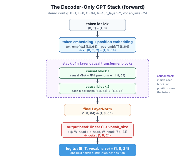
The forward pass reuses the exact layers you already wrote. The only new piece is that multi-head attention now applies the causal mask, so we write a causal_multi_head_attention that is the Module 5 attention with the mask from Lesson 2 folded in. Everything else — layer norm, the GELU feed-forward network, the pre-norm block — is unchanged.

import numpy as np

def softmax(x, axis=-1):
    x = x - x.max(axis=axis, keepdims=True)   # subtract row max for stability
    e = np.exp(x)
    return e / e.sum(axis=axis, keepdims=True)

def causal_multi_head_attention(X, Wq, Wk, Wv, Wo, h):
    B, T, C = X.shape
    hs = C // h
    Q = (X @ Wq).reshape(B, T, h, hs).transpose(0, 2, 1, 3)
    K = (X @ Wk).reshape(B, T, h, hs).transpose(0, 2, 1, 3)
    V = (X @ Wv).reshape(B, T, h, hs).transpose(0, 2, 1, 3)
    scores = Q @ K.transpose(0, 1, 3, 2) / np.sqrt(hs)   # (B, h, T, T)
    mask = np.triu(np.ones((T, T), dtype=bool), k=1)     # True strictly above the diagonal
    scores = np.where(mask, -1e9, scores)                # forbid attending to the future
    weights = softmax(scores, axis=-1)                   # (B, h, T, T)
    per_head = weights @ V                               # (B, h, T, hs)
    concat = per_head.transpose(0, 2, 1, 3).reshape(B, T, C)
    return concat @ Wo                                   # (B, T, C)

def layer_norm(x, gamma, beta, eps=1e-5):
    mu  = x.mean(axis=-1, keepdims=True)
    var = x.var(axis=-1, keepdims=True)
    xhat = (x - mu) / np.sqrt(var + eps)
    return gamma * xhat + beta

def gelu(x):
    return 0.5 * x * (1.0 + np.tanh(np.sqrt(2.0 / np.pi) * (x + 0.044715 * x**3)))

def feed_forward(x, W1, b1, W2, b2):
    hidden = gelu(x @ W1 + b1)
    return hidden @ W2 + b2

The causal block is the pre-norm block from Module 5, calling causal_multi_head_attention for its first sublayer. Two sublayers, each normalized on the way in and wrapped in a residual add.

def causal_block_forward(x, p):
    # Sublayer 1: causal multi-head attention, pre-norm, residual
    ln1  = layer_norm(x, p["ln1_gamma"], p["ln1_beta"])
    attn = causal_multi_head_attention(ln1, p["Wq"], p["Wk"], p["Wv"], p["Wo"], p["h"])
    x    = x + attn
    # Sublayer 2: feed-forward network, pre-norm, residual
    ln2  = layer_norm(x, p["ln2_gamma"], p["ln2_beta"])
    ff   = feed_forward(ln2, p["W1"], p["b1"], p["W2"], p["b2"])
    return x + ff

Nothing above is new machinery; it is the code you have run in earlier lessons, gathered in one place so the model that follows has all its parts.

Building the Model’s Parameters#

A GPT owns three kinds of parameters: the two embedding tables, the per-block weights (one set per block in the stack), and the final layer norm plus the output head. We build each block with the same helper from Module 5, and gather the rest into one params dictionary. We seed with default_rng(42) and use the standard * 0.02 init, since this lesson inspects shapes, not attention patterns.

def make_block_params(rng, C, h):
    return dict(
        Wq=rng.standard_normal((C, C)) * 0.02,
        Wk=rng.standard_normal((C, C)) * 0.02,
        Wv=rng.standard_normal((C, C)) * 0.02,
        Wo=rng.standard_normal((C, C)) * 0.02,
        ln1_gamma=np.ones(C), ln1_beta=np.zeros(C),
        ln2_gamma=np.ones(C), ln2_beta=np.zeros(C),
        W1=rng.standard_normal((C, 4 * C)) * 0.02, b1=np.zeros(4 * C),
        W2=rng.standard_normal((4 * C, C)) * 0.02, b2=np.zeros(C),
        h=h,
    )

def make_gpt_params(rng, vocab_size, block_size, C, h, n_layer):
    return dict(
        tok_emb=rng.standard_normal((vocab_size, C)) * 0.02,   # token embedding table
        pos_emb=rng.standard_normal((block_size, C)) * 0.02,   # position embedding table
        blocks=[make_block_params(rng, C, h) for _ in range(n_layer)],
        lnf_gamma=np.ones(C), lnf_beta=np.zeros(C),            # final layer norm
        W_head=rng.standard_normal((C, vocab_size)) * 0.02,    # output head: C -> vocab_size
        b_head=np.zeros(vocab_size),
    )

Notice the two embedding tables. tok_emb has one row per vocabulary entry, shape (vocab_size, C); indexing it with a token id returns that token’s vector. pos_emb has one row per position up to block_size, shape (block_size, C); we take the first $T$ rows for a sequence of length $T$. The output head W_head has shape (C, vocab_size): it maps a width-$C$ vector to one score per vocabulary entry, the mirror image of the token embedding table’s shape.

Writing gpt_forward#

Now the model itself. gpt_forward walks the four stages in order: embed, run the block stack, apply the final layer norm, and project to logits. The verbose flag prints the shape at every stage so you can watch (B, T) grow into (B, T, C) and then collapse to (B, T, vocab_size).

def gpt_forward(idx, p, verbose=False):
    B, T = idx.shape
    # Stage 1: embeddings
    tok = p["tok_emb"][idx]     # (B, T, C)  look up a vector per token id
    pos = p["pos_emb"][:T]      # (T, C)     first T position vectors
    x = tok + pos               # (B, T, C)  broadcast the positions over the batch
    if verbose:
        print("token ids idx     :", idx.shape, "(B, T)")
        print("token embeddings  :", tok.shape, "(B, T, C)")
        print("position emb (:T) :", pos.shape, "(T, C)")
        print("embedded x        :", x.shape, "(B, T, C)")
    # Stage 2: the stack of causal transformer blocks
    for i, bp in enumerate(p["blocks"]):
        x = causal_block_forward(x, bp)
        if verbose:
            print("after block %d     :" % (i + 1), x.shape, "(B, T, C)")
    # Stage 3: final layer norm
    x = layer_norm(x, p["lnf_gamma"], p["lnf_beta"])
    if verbose:
        print("after final LN    :", x.shape, "(B, T, C)")
    # Stage 4: output head -> logits
    logits = x @ p["W_head"] + p["b_head"]   # (B, T, vocab_size)
    if verbose:
        print("logits            :", logits.shape, "(B, T, vocab_size)")
    return logits

The body is a direct reading of the pipeline. p["tok_emb"][idx] is the fancy-indexing lookup: an integer array of shape (B, T) indexing a (vocab_size, C) table yields (B, T, C). Adding pos of shape (T, C) broadcasts it across the batch. The for loop is the stack: each pass overwrites x with the block’s output, and because every block preserves shape, the loop can run any number of times. The final layer norm and the matrix multiply by W_head finish the job.

Running the Forward Pass#

Time to run it. We use a small config for speed: width $C = 64$ with $h = 4$ heads, a stack of $n\_layer = 2$ blocks, block_size = 16, and vocab_size = 24 (the size of our char-level vocabulary). We feed a single sequence of eight token ids, $B = 1$, $T = 8$, and print the shape at every stage.

rng = np.random.default_rng(42)
vocab_size, block_size = 24, 16
C, h, n_layer = 64, 4, 2
B, T = 1, 8

params = make_gpt_params(rng, vocab_size, block_size, C, h, n_layer)
idx = rng.integers(0, vocab_size, size=(B, T))

print("config: vocab_size=%d, block_size=%d, C=%d, h=%d, n_layer=%d"
      % (vocab_size, block_size, C, h, n_layer))
print("input token ids   :", idx.tolist())
print("-" * 46)
logits = gpt_forward(idx, params, verbose=True)
print("-" * 46)
print("final logits shape:", logits.shape)
print("expected          : (1, 8, 24)")

config: vocab_size=24, block_size=16, C=64, h=4, n_layer=2
input token ids   : [[20, 17, 9, 15, 22, 17, 12, 19]]
----------------------------------------------
token ids idx     : (1, 8) (B, T)
token embeddings  : (1, 8, 64) (B, T, C)
position emb (:T) : (8, 64) (T, C)
embedded x        : (1, 8, 64) (B, T, C)
after block 1     : (1, 8, 64) (B, T, C)
after block 2     : (1, 8, 64) (B, T, C)
after final LN    : (1, 8, 64) (B, T, C)
logits            : (1, 8, 24) (B, T, vocab_size)
----------------------------------------------
final logits shape: (1, 8, 24)
expected          : (1, 8, 24)

Trace the shapes down the output. The token ids came in as (1, 8). The embeddings lifted them to (1, 8, 64) by attaching a width-64 vector to each token. Both blocks preserved (1, 8, 64), exactly as the shape-preserving property promises, so the stack could be two blocks or twenty without changing the interface. The final layer norm kept (1, 8, 64), and the output head projected the width-64 axis down to vocab_size, giving (1, 8, 24). That is a full GPT forward pass.

Checking the Logits Are Valid Predictions#

The shape is right, but are these logits actually usable as next-token predictions? Each position’s slice, logits[0, t], is a length-24 vector of raw scores. To be a valid pre-softmax vector it only needs to be finite real numbers of the right length; applying softmax must then produce a proper probability distribution — non-negative entries that sum to 1. Let’s confirm that for every position.

probs = softmax(logits, axis=-1)          # (1, 8, 24)
row_sums = probs.sum(axis=-1)             # (1, 8)
print("softmax row sums  :", np.round(row_sums[0], 6).tolist())
print("all rows sum to 1?", np.allclose(row_sums, 1.0))
print("logits[0, 0, :5]  :", np.round(logits[0, 0, :5], 6).tolist())
print("argmax next-token per position:", logits.argmax(axis=-1)[0].tolist())

softmax row sums  : [1.0, 1.0, 1.0, 1.0, 1.0, 1.0, 1.0, 1.0]
all rows sum to 1? True
logits[0, 0, :5]  : [-0.125102, -0.162544, 0.013865, 0.063748, 0.057978]
argmax next-token per position: [5, 19, 20, 23, 7, 12, 10, 12]

All eight positions produce a distribution that sums to 1, so each is a valid next-token prediction over the 24-character vocabulary. The argmax line reads out the single most likely next token at each position: position 0 predicts token 5 as most likely, position 1 predicts token 19, and so on, one prediction per position. These predictions are meaningless right now, of course, because the weights are random and untrained. But the machinery is complete and correct: given a context, the model emits a probability distribution over what comes next, at every position, in one pass.

To confirm there is no hidden randomness, run the whole script a second time. Because every random draw is seeded with default_rng(42), the token ids, the logits, and the argmax are byte-for-byte identical across runs — this course has no nondeterminism.

Practice Exercises#

Try these before checking the hints. They reuse gpt_forward, make_gpt_params, and the demo variables above.

Exercise 1: Grow the Stack#

Rebuild the parameters with n_layer = 6 instead of 2, keeping everything else the same, and run gpt_forward on the same idx. Confirm the final logits are still (1, 8, 24), and note how many “after block” lines print now.

# Your code here: make_gpt_params(..., n_layer=6), then gpt_forward(idx, params, verbose=True)

Exercise 2: Batch Several Sequences#

Feed a batch of B = 4 sequences of length T = 8 at once (rng.integers(0, vocab_size, size=(4, 8))). Print the logits shape and verify every position in every sequence gives a distribution that sums to 1.

# Your code here: build idx of shape (4, 8), run gpt_forward, softmax and check row sums

Exercise 3: Tie the Output Head to the Embeddings#

Instead of a separate W_head, project with the transpose of the token embedding table: replace x @ p["W_head"] + p["b_head"] with x @ p["tok_emb"].T. Confirm the logits shape is unchanged and explain in a comment why the shapes line up.

# Your code here: a copy of gpt_forward whose head is x @ p["tok_emb"].T

Summary#

You assembled a complete GPT forward pass. Starting from a batch of token ids, you embedded them, ran them through a stack of causal transformer blocks, normalized once, and projected to a distribution over the vocabulary at every position. Let’s review.

Key Concepts#

Decoder-Only

• The original transformer had an encoder and a decoder; GPT keeps only the decoder stack and drops cross-attention, leaving uniform blocks of causal self-attention plus a feed-forward network
• “Decoder” is a statement about time: generation is left to right, and the causal mask in every block enforces the no-peeking rule at every layer

The Four Stages

• Embeddings: tok_emb[idx] + pos_emb[:T] turns ids (B, T) into activations (B, T, C)
• Causal block stack: n_layer blocks, each mapping (B, T, C) to (B, T, C), so depth never changes the shape
• Final layer norm: cleans up the un-normalized output of the last pre-norm block
• Output head: a linear map (C to vocab_size) producing logits (B, T, vocab_size)

The Output

• Logits have shape (B, T, vocab_size); each position’s slice is a valid pre-softmax vector whose softmax sums to 1
• The model emits one next-token distribution per position, all in a single parallel forward pass
• Weight tying is an option: reuse tok_emb.T as the output head to share parameters

Verification

• The demo turned ids (1, 8) into logits (1, 8, 24); softmax row sums were all 1.0 across every position
• With default_rng(42), two runs produce byte-for-byte identical logits — no nondeterminism

Why This Matters#

This is the architecture. Every GPT you have heard of, from the smallest research model to the largest production system, is this same decoder-only stack: embed, run causal blocks, normalize, project to vocabulary logits. The only differences are scale — more layers, wider models, bigger vocabularies, longer contexts — and refinements to the individual pieces. The skeleton you wrote in a few dozen lines of NumPy is the real skeleton.

Seeing the forward pass hold together shape-for-shape also changes how you read a model. When a config lists n_layer, n_embd, n_head, block_size, and vocab_size, you now know exactly where each number lives: how many times the block loop runs, how wide the activations are, how attention splits, how far positions reach, and how large the final projection is. A GPT stops being a black box and becomes a pipeline you can trace with your finger.

Continue Building Your Skills#

You now have a model that maps token ids to next-token logits, but it has no way to know whether those predictions are any good. That is the missing piece the next lesson supplies. In Lesson 4 you will build the language-modeling head’s loss: take the logits at each position, compare them against the true next token with softmax cross-entropy, and average into a single scalar that measures how surprised the model was by the real continuation. That one number is what training will drive downward. You will compute it in NumPy on the Lantern Bay corpus, watch what an untrained model’s loss looks like against the vocabulary size, and set up exactly the quantity whose gradient Lesson 5 sends back through the entire stack you just assembled.