Lesson 4 - The Language-Modeling Head & Loss

Welcome to The Language-Modeling Head & Loss#

In the last three lessons you built the body of a GPT: token and position embeddings feed a stack of causal transformer blocks, and out comes a tensor of hidden states shaped (B, T, C), one C-dimensional vector summarizing what the model knows at each position. That tensor is rich, but it is not yet an answer. A language model has exactly one job: at every position, predict the next token. This lesson adds the two pieces that turn hidden states into that prediction and, crucially, into a single number you can train against.

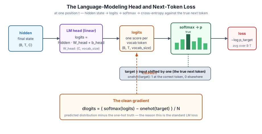
The first piece is the language-modeling head, a plain linear layer that projects each hidden vector to one score per vocabulary token. The second is the loss: softmax those scores into a probability distribution over the vocabulary, and measure how much probability the model put on the token that actually came next. Averaged over every position in the batch, that is the softmax cross-entropy next-token loss, the objective every GPT is trained on. Its gradient turns out to be one of the cleanest results in deep learning, softmax(logits) - onehot(target), and by the end of this lesson you will have derived it, implemented it, and proven it correct against a numerical gradient check.

By the end of this lesson, you will be able to:

• Add a linear LM head that maps hidden states (B, T, C) to logits (B, T, vocab_size)
• Explain why the next-token target is simply the input sequence shifted by one
• Write the softmax cross-entropy loss as the average negative log-probability of the true next token
• Derive the clean softmax - onehot gradient of the loss with respect to the logits
• Implement cross_entropy_loss returning both the loss and dlogits, and backprop through the head to dW_head, db_head, and dhidden
• Verify every gradient against a float64 finite-difference check and confirm a random model scores the uniform baseline

You should be comfortable with the causal transformer stack from the earlier lessons in this module and with the softmax cross-entropy gradient idea from the foundations course. Let’s begin.

From Hidden States to Vocabulary Scores#

The transformer stack hands you hidden, a (B, T, C) tensor. B is the batch of sequences, T is the sequence length, and C = n_embd is the model width. Each of the B * T positions carries a C-dimensional vector, but to predict a token we need a score for every entry in the vocabulary, not a C-dimensional summary. The language-modeling head bridges that gap with a single linear layer:

Here W_head has shape (C, vocab_size) and b_head has shape (vocab_size,). The matrix multiply contracts the C axis and replaces it with vocab_size, so logits comes out shaped (B, T, vocab_size): at every position, one raw, unnormalized score per vocabulary token. A high logit for the character t at position 5 means the model currently favors t as the token following position 5. These scores are not yet probabilities, they can be any real number, positive or negative; turning them into a distribution is the softmax’s job in the next section.

The Next-Token Target Is the Input, Shifted by One#

Before we can score a prediction we need to know the right answer at every position. In language modeling the right answer is delightfully cheap: the token that actually followed. If the input at position t is x[t], the target the model should predict there is x[t+1]. So the target sequence is just the input sequence shifted left by one. No labels to collect, no annotation, the text is its own supervision. This is what makes language modeling scale: any text is training data.

Concretely, if the input row is x = data[i : i+T], the matching targets are y = data[i+1 : i+T+1]. Position 0 of the input should predict position 0 of the targets (which is the input’s position 1), and so on down the sequence. Every one of the T positions produces a prediction and has a target, so a single (B, T) batch gives B * T independent next-token predictions to learn from at once, which is exactly the parallelism the causal mask made safe in Lesson 2.

Let’s set up the corpus, tokenize it at the character level, and pull one batch so the targets are concrete.

import numpy as np

# ----- corpus & char tokenization (canonical for this course) -----
CORPUS = (
    "the lamp keeper walks the shore at dusk. "
    "the lamp keeper lights the lantern when the fog rolls in. "
    "the boats come home when the lantern glows. "
    "the boats wait outside the bay when the fog is thick. "
    "a small boat drifts near the rocks at dawn. "
    "the keeper rings the bell when a boat drifts near the rocks. "
    "the tide rises at dusk and falls at dawn. "
    "the gulls call over the bay when the tide is low. "
    "the keeper counts the boats and writes the count in a book. "
    "the lantern burns all night and rests at dawn. "
) * 20

chars = sorted(set(CORPUS))
vocab_size = len(chars)
stoi = {c: i for i, c in enumerate(chars)}
itos = {i: c for i, c in enumerate(chars)}
encode = lambda s: [stoi[c] for c in s]
decode = lambda ids: "".join(itos[i] for i in ids)
data = np.array(encode(CORPUS), dtype=np.int64)

# ----- one batch: targets are inputs shifted by one -----
rng = np.random.default_rng(42)
B, T, C = 4, 8, 16          # tiny demo: batch 4, context 8, width 16
block_size = T
ix = rng.integers(0, len(data) - block_size - 1, size=B)
xb = np.stack([data[i:i + T] for i in ix])          # (B, T) input tokens
yb = np.stack([data[i + 1:i + T + 1] for i in ix])  # (B, T) next-token targets

print("vocab_size:", vocab_size, " len(data):", len(data))
print("xb:", xb.shape, " yb:", yb.shape)
print("input :", repr(decode(xb[0])))
print("target:", repr(decode(yb[0])))

vocab_size: 24  len(data): 10020
xb: (4, 8)  yb: (4, 8)
input : '. the ke'
target: ' the kee'

The vocabulary is 24 characters (lowercase letters, space, and a period) and the encoded corpus is 10020 tokens, exactly as the course expects. Look at the first row: the input '. the ke' and the target ' the kee' are the same text offset by one character. Where the input reads ., the target reads a space; where the input reads e, the target reads the next e. Predicting the target from the input is predicting the next character, position by position.

Softmax, Then the Negative Log-Probability of the Truth#

Now score the batch. We use a (B, T, C) tensor of random hidden states to stand in for the output of an untrained stack, add the LM head, and get logits. Because the head is initialized small (* 0.02), the logits are all near zero, which makes the softmax nearly uniform, exactly the state an untrained model should be in.

def softmax(x, axis=-1):
    x = x - x.max(axis=axis, keepdims=True)   # stable: subtract row max
    e = np.exp(x)
    return e / e.sum(axis=axis, keepdims=True)

# final hidden states from a (pretend) untrained stack, plus the LM head
hidden = rng.standard_normal((B, T, C))               # (B, T, C)
W_head = rng.standard_normal((C, vocab_size)) * 0.02  # (C, vocab_size)
b_head = np.zeros(vocab_size)                          # (vocab_size,)

logits = hidden @ W_head + b_head                      # (B, T, vocab_size)
print("logits:", logits.shape, " dtype:", logits.dtype)

logits: (4, 8, 24)  dtype: float64

Each of the 4 * 8 = 32 positions now has 24 logits, one per vocabulary token, and everything is float64 so the gradient check later has the precision to trust. To turn logits into a loss, do two things at every position t: softmax the 24 logits into a probability distribution $p$ over the vocabulary, then read off $p$ at the true next token and take its negative logarithm. If the model gave the correct token high probability, $-\log p_{\text{target}}$ is small; if it gave it near-zero probability, the loss shoots up. Averaging that penalty over all $N = B \cdot T$ positions is the softmax cross-entropy next-token loss:

The cross_entropy_loss function below computes exactly this. It flattens the (B, T, V) logits to (N, V) so the two batch axes collapse into one list of N independent predictions, softmaxes each row, gathers the probability at each row’s target token, and averages the negative logs. It also returns the gradient we are about to derive, so the forward and backward live together.

def cross_entropy_loss(logits, targets):
    # logits: (B, T, V);  targets: (B, T) int64
    B, T, V = logits.shape
    N = B * T
    flat = logits.reshape(N, V)
    tgt = targets.reshape(N)
    probs = softmax(flat, axis=-1)                  # (N, V)
    logp = np.log(probs[np.arange(N), tgt])         # (N,) log-prob of the true token
    loss = -np.mean(logp)
    # gradient: (softmax - onehot) / N  (derived below)
    dflat = probs.copy()
    dflat[np.arange(N), tgt] -= 1.0
    dflat /= N
    dlogits = dflat.reshape(B, T, V)
    return loss, dlogits

loss, dlogits = cross_entropy_loss(logits, targets=yb)
print("loss:", round(float(loss), 6))
print("log(vocab_size):", round(float(np.log(vocab_size)), 6))
print("dlogits:", dlogits.shape)

loss: 3.179347
log(vocab_size): 3.178054
dlogits: (4, 8, 24)

The loss is 3.179347, essentially identical to $\log(\text{vocab\_size}) = \log 24 \approx 3.178$. That is not a coincidence, and it is the single most useful sanity check in this whole course.

The Gradient: Why It Collapses to softmax minus onehot#

The reason softmax cross-entropy is the language-modeling loss is not only that it measures the right thing, it is that its gradient with respect to the logits is astonishingly clean. Consider a single position with logits $z$ (a vector of length vocab_size), softmax probabilities $p = \text{softmax}(z)$, and true token index $c$. The per-position loss is $\ell = -\log p_c$.

Two derivatives combine. First, the loss depends on the logits only through $p_c$, and $\ell = -\log p_c$ gives $\partial \ell / \partial p_c = -1/p_c$. Second, the softmax has the Jacobian $\partial p_i / \partial z_j = p_i(\delta_{ij} - p_j)$, where $\delta_{ij}$ is 1 when $i = j$ and 0 otherwise. Chaining them, the gradient on logit $j$ is

Every term collapses because the only non-zero $\partial \ell / \partial p_i$ is at $i = c$. The result, $p_j - \delta_{cj}$, is simply the softmax probability minus 1 at the true token and unchanged everywhere else, that is, softmax(z) - onehot(c). Because the batch loss averages over $N$ positions, each position’s gradient carries a factor of $1/N$:

That is the entire backward through the loss, and it is exactly the three lines inside cross_entropy_loss: take probs, subtract 1 at each row’s target column, and divide by N. Intuitively the gradient says push the probability of the correct token up and every other token’s probability down, with the size of each push proportional to how much probability is currently misplaced. No logarithms, no divisions, no softmax Jacobian survive into the code, which is why this loss is both numerically stable and the universal choice for classifiers and language models alike.

Proving the Loss Gradient with a Numerical Check#

A clean formula is not a proof. As with every backward pass in this course, we confirm dlogits numerically: nudge a single logit up by a tiny $\epsilon$, nudge it down by $\epsilon$, see how much the loss moved, and divide. This central finite difference must match the analytic gradient for every entry.

def num_grad_logits(logits, targets, eps=1e-6):
    g = np.zeros_like(logits)
    it = np.nditer(logits, flags=["multi_index"])
    while not it.finished:
        idx = it.multi_index
        orig = logits[idx]
        logits[idx] = orig + eps
        Lp, _ = cross_entropy_loss(logits, targets)
        logits[idx] = orig - eps
        Lm, _ = cross_entropy_loss(logits, targets)
        logits[idx] = orig                    # always restore the entry
        g[idx] = (Lp - Lm) / (2 * eps)
        it.iternext()
    return g

def max_rel_err(a, n):
    denom = np.maximum(np.abs(a), np.abs(n)) + 1e-12
    return np.max(np.abs(a - n) / denom)

num_dlogits = num_grad_logits(logits.copy(), yb)
print("dlogits max rel err :", max_rel_err(dlogits, num_dlogits))
print("softmax-minus-onehot == numerical:", np.allclose(dlogits, num_dlogits, atol=1e-7))

dlogits max rel err : 2.373624716282666e-07
softmax-minus-onehot == numerical: True

The max relative error is about $2.4 \times 10^{-7}$, far below the $10^{-4}$ bar that separates a correct gradient from a buggy one, and np.allclose confirms the analytic softmax - onehot result matches the brute-force perturbation everywhere. The famously simple formula is not a shortcut that trades away correctness; it is exactly the gradient, and now you have proof.

Backprop Through the Head: dW_head, db_head, dhidden#

dlogits is the gradient entering the LM head from the loss. The head itself is a plain linear layer, logits = hidden @ W_head + b_head, so its backward pass is the same dense-layer rule you used in the foundations course, applied with hidden as the input. Flatten the two batch axes into one so the multiply is an ordinary matrix product over N = B * T rows:

W_head is shared across every position, so its gradient sums the contributions of all N rows; b_head was added to every row, so its gradient sums dlogits over those rows; and dhidden flows back to the stack below with W_head transposed, ready to continue the backward pass through the transformer blocks.

N = B * T
dW_head = hidden.reshape(N, C).T @ dlogits.reshape(N, vocab_size)  # (C, vocab_size)
db_head = dlogits.reshape(N, vocab_size).sum(axis=0)              # (vocab_size,)
dhidden = dlogits @ W_head.T                                      # (B, T, C)

print("dW_head:", dW_head.shape, " db_head:", db_head.shape, " dhidden:", dhidden.shape)

dW_head: (16, 24)  db_head: (24,)  dhidden: (4, 8, 16)

Each gradient matches the shape of the quantity it belongs to: dW_head is (C, vocab_size) = (16, 24) like W_head, db_head is (24,) like b_head, and dhidden is (B, T, C) = (4, 8, 16) like the hidden states. That shape agreement is the first check; the numerical check is the real one. We gradient-check the two head parameters by perturbing their entries and comparing to the analytic gradients.

def loss_from_params(W_head, b_head):
    lg = hidden @ W_head + b_head
    L, _ = cross_entropy_loss(lg, yb)
    return L

def num_grad_param(param, eps=1e-6):
    g = np.zeros_like(param)
    it = np.nditer(param, flags=["multi_index"])
    while not it.finished:
        idx = it.multi_index
        orig = param[idx]
        param[idx] = orig + eps
        Lp = loss_from_params(W_head, b_head)
        param[idx] = orig - eps
        Lm = loss_from_params(W_head, b_head)
        param[idx] = orig
        g[idx] = (Lp - Lm) / (2 * eps)
        it.iternext()
    return g

print("dW_head max rel err:", max_rel_err(dW_head, num_grad_param(W_head)))
print("db_head max rel err:", max_rel_err(db_head, num_grad_param(b_head)))

dW_head max rel err: 3.2679370812059283e-06
db_head max rel err: 2.351571740810997e-08

Both errors sit between $10^{-6}$ and $10^{-8}$, comfortably below the $10^{-4}$ threshold. The LM head’s backward pass is correct: from a single scalar loss you have produced a gradient for W_head, for b_head, and for the hidden states feeding in, each verified against a numerical estimate. Because every random draw is seeded with default_rng(42) and the finite-difference loop is deterministic, running the whole script a second time prints byte-for-byte identical numbers, this course has no nondeterminism to worry about.

Practice Exercises#

Try these before checking the hints. They reuse cross_entropy_loss, softmax, num_grad_logits, max_rel_err, and the tensors (hidden, W_head, b_head, xb, yb) defined above.

Exercise 1: Make the Loss Nearly Zero#

A confident, correct model should have a loss near zero. Construct logits that put almost all probability on the true target at every position, then confirm cross_entropy_loss returns a value close to 0. Start from logits and add a large positive number at each position’s target token.

# Your code here: build "confident" logits that spike at the true target,
# then print the resulting loss

Exercise 2: Check That dlogits Sums to Zero Per Position#

The gradient softmax - onehot has a hidden structure: at each position the softmax probabilities sum to 1 and the one-hot sums to 1, so their difference sums to 0. Verify that each position’s slice of dlogits sums to (essentially) zero across the vocabulary axis.

# Your code here: sum dlogits over the vocab axis and check it is ~0 everywhere

Exercise 3: Confirm the Uniform Baseline Directly#

The lesson claimed a random model scores about $\log(\text{vocab\_size})$. Prove it without any model at all: set every logit to the same constant so the softmax is exactly uniform, and check the loss equals $\log 24$ to machine precision, for any targets.

# Your code here: build all-equal logits, run cross_entropy_loss, compare to log(vocab_size)

Summary#

You built the final component that turns a transformer body into a trainable language model: the head that produces vocabulary scores and the loss that grades them. Let’s review.

Key Concepts#

The LM Head

• A linear layer logits = hidden @ W_head + b_head with W_head shaped (C, vocab_size), mapping hidden states (B, T, C) to logits (B, T, vocab_size)
• One raw score per vocabulary token at every position; not yet probabilities
• Often weight-tied with the token embedding table, which has the transposed shape

The Next-Token Loss

• The target is the input shifted by one: predict x[t+1] at position t, so text supervises itself
• Softmax each position’s logits into a distribution, then take $-\log p_{\text{target}}$; average over all $N = B \cdot T$ positions: $L = -\frac{1}{N}\sum \log p_{\text{target}}$
• A random model scores the uniform baseline $\log(\text{vocab\_size}) = \log 24 \approx 3.178$; the loss falling below it is the first sign of learning

The Clean Gradient

• Softmax and cross-entropy collapse to $\frac{\partial L}{\partial \text{logits}} = \frac{1}{N}(\text{softmax}(\text{logits}) - \text{onehot}(\text{target}))$, computed in three lines
• The head backward is a dense layer: dW_head = hiddenᵀ @ dlogits, db_head = dlogits.sum(0), dhidden = dlogits @ W_headᵀ
• Real max relative errors were 2e-7 (dlogits), 3e-6 (dW_head), and 2e-8 (db_head), all far below 1e-4, and identical on re-run

Why This Matters#

The softmax cross-entropy next-token loss is the objective behind every GPT ever trained, and its softmax - onehot gradient is one of those rare results where the math and the code line up so cleanly that it feels like a trick. It is not a trick, it is the exact gradient, and you proved it against a numerical check rather than taking it on faith. That habit, deriving a gradient and then verifying it, is what lets you build custom losses and layers with confidence instead of hope.

Just as important, this lesson is where the model’s backward pass starts. The loss produces dlogits, the head turns it into dhidden, and dhidden is the gradient that will flow down through the final norm, the causal blocks, and the embeddings to train the entire network. You have now built every forward and backward piece of a GPT in isolation. The only thing left is to wire them together.

Continue Building Your Skills#

Every part is now on the table: token and position embeddings, causal transformer blocks, a final layer norm, and, as of this lesson, the language-modeling head with a gradient-checked next-token loss. In the next lesson, the module’s guided project, you will assemble them into one complete mini-GPT class, a model that takes a batch of token ids, runs embeddings into a stack of causal blocks into the final norm into the head, and returns both the loss and a full set of gradients. You will thread dlogits from cross_entropy_loss back through the head to dhidden, then down through every block you built earlier, and gradient-check the assembled model end to end. When that check passes, you will have a real GPT in pure NumPy, forward and backward, ready for the training loop in Module 7 where the loss you built today finally starts to fall below 3.178.