Lesson 1 - The Limits of Recurrence

Welcome to The Limits of Recurrence#

Over this course you’ll build a small character-level GPT from nothing but NumPy — one component at a time — until it can read the Lantern Bay corpus and generate text in the same style. Before you write a single line of attention, though, it’s worth understanding why that model is built the way it is. Every design choice in a transformer is a reaction to something that came before: the recurrent neural network, or RNN, the workhorse that dominated sequence modeling for years.

This lesson has no attention code yet — that arrives in Lesson 2. Instead, you’ll build a real RNN in NumPy, run it, and watch it hit three walls. Feeling those walls in actual numbers is the best possible motivation for the machinery you’re about to construct.

By the end of this lesson, you will be able to:

• Describe how an RNN processes a sequence one step at a time through a single hidden state
• Implement a tiny RNN forward pass in NumPy and confirm its hidden state is a fixed-size vector regardless of sequence length
• Explain the three core limits of recurrence: sequential computation, the fixed-size memory bottleneck, and fading long-range signal
• Measure signal decay directly by perturbing the first token and watching its influence shrink over many steps
• State, at a high level, how attention removes all three limits at once

You should be comfortable with NumPy arrays, matrix multiplication, and the idea of a hidden layer from earlier deep-learning work. Let’s begin by looking at how a recurrent network actually reads.

How an RNN Reads a Sequence#

A recurrent network processes a sequence the way you might read a sentence with a very short memory: one token at a time, updating a single running summary as you go. That running summary is the hidden state $h_t$, a fixed-size vector. At each step the RNN combines the current input $x_t$ with the previous hidden state $h_{t-1}$ to produce a new hidden state:

Here $W_x$ maps the input into the hidden space, $W_h$ maps the previous hidden state forward, $b$ is a bias, and $\tanh$ squashes everything into $(-1, 1)$. The starting state $h_0$ is usually all zeros. Read that formula carefully and two facts jump out. First, $h_t$ depends on $h_{t-1}$, which depends on $h_{t-2}$, and so on — the computation is a strict chain. Second, no matter how long the sequence is, everything the model knows about the entire past is carried in that one vector $h_t$.

Those two facts are the seeds of the three limits we’re about to measure. Let’s make the network real.

A Tiny RNN in NumPy#

We’ll build the smallest RNN that shows the behavior clearly: an input of width 8 and a hidden state of width 16. Small random weights, a fixed seed, and pure NumPy — no framework anywhere.

import numpy as np

np.random.seed(42)

C_in = 8     # input feature size
H = 16       # hidden size (fixed)

Wx = np.random.randn(H, C_in) * 0.3   # input  -> hidden
Wh = np.random.randn(H, H) * 0.3      # hidden -> hidden
b  = np.zeros(H)

def rnn_forward(xs, h0=None):
    """xs: (T, C_in). Returns hidden states stacked as (T, H)."""
    h = np.zeros(H) if h0 is None else h0
    hs = []
    for t in range(xs.shape[0]):
        h = np.tanh(Wx @ xs[t] + Wh @ h + b)   # h_t = tanh(Wx x_t + Wh h_{t-1} + b)
        hs.append(h)
    return np.array(hs)

The function is a direct transcription of the formula: a Python for loop that walks the sequence, and inside it a single line that turns $x_t$ and the previous h into the next h. That loop is not an implementation detail — it is the recurrence, and we’ll come back to it. Now run a short sequence of length 5 through it and print the hidden-state shape at every step.

T = 5
xs = np.random.randn(T, C_in)
hs = rnn_forward(xs)

for t in range(T):
    print(f"step {t}: h_t shape = {hs[t].shape}")
print("all hidden states stacked:", hs.shape)

step 0: h_t shape = (16,)
step 1: h_t shape = (16,)
step 2: h_t shape = (16,)
step 3: h_t shape = (16,)
step 4: h_t shape = (16,)
all hidden states stacked: (5, 16)

Every hidden state is a vector of shape (16,). The RNN produced one summary per step, each the same fixed width. Now the important question: what happens to that width if the sequence gets much longer?

xs_long = np.random.randn(40, C_in)
hs_long = rnn_forward(xs_long)

print("length-40 sequence, final h shape =", hs_long[-1].shape)
print("same fixed width regardless of T:", hs[-1].shape == hs_long[-1].shape)

length-40 sequence, final h shape = (16,)
same fixed width regardless of T: True

A sequence eight times longer still ends in a hidden state of exactly 16 numbers. This is the fixed-size memory bottleneck in the flesh: whether the model has read 5 tokens or 40 or 40,000, the entire memory of the past is compressed into the same 16-dimensional vector. There is nowhere else for information to live.

Limit 1: Computation Must Be Sequential#

Look again at that for loop. To compute hs[4] you first need hs[3], which needs hs[2], and so on back to hs[0]. Step $t$ genuinely cannot start until step $t-1$ has finished, because $h_{t-1}$ is one of its inputs. The recurrence is a data dependency, and it forces the whole sequence to be processed strictly in order.

This is a problem on modern hardware. GPUs are fast because they do thousands of operations at the same time, but you cannot parallelize a chain where each link waits for the previous one. A 1,000-token sequence means 1,000 steps that must run back to back. Let’s count the dependency directly and contrast it with what attention will offer — a comparison of all positions at once, with no ordering constraint.

import numpy as np

for T in [8, 32, 128]:
    rnn_serial_steps  = T          # must run t = 0..T-1 strictly in order
    attn_pairs        = T * T      # every position compares to every position
    longest_path_rnn  = T          # token 0 -> token T-1 crosses T-1 hops
    longest_path_attn = 1          # token 0 reaches token T-1 in a single hop
    print(f"T={T:3d} | RNN ordered steps={rnn_serial_steps:3d} "
          f"(longest path {longest_path_rnn:3d} hops) | "
          f"attention pairs={attn_pairs:5d} (longest path {longest_path_attn} hop)")

T=  8 | RNN ordered steps=  8 (longest path   8 hops) | attention pairs=   64 (longest path 1 hop)
T= 32 | RNN ordered steps= 32 (longest path  32 hops) | attention pairs= 1024 (longest path 1 hop)
T=128 | RNN ordered steps=128 (longest path 128 hops) | attention pairs=16384 (longest path 1 hop)

The RNN column grows linearly and, crucially, those steps cannot overlap. Attention does more raw comparisons — all $T^2$ pairs — but there is no ordering between them, so they can all be computed in parallel in a single matrix multiply. Notice the “longest path” column too: in an RNN, information from the first token has to travel through $T-1$ intermediate hidden states to reach the last one. In attention, it’s always one hop. That short path is exactly what fixes the next limit.

Limit 2 and 3: The Signal From Early Tokens Fades#

The longest-path count hinted at the deepest problem. When information from token 0 must pass through many tanh updates to reach a distant step, it decays along the way — and so does the gradient that would train the early weights. This is the famous vanishing signal (and vanishing gradient) of deep recurrence. Instead of taking it on faith, let’s measure it.

The experiment is simple. Run the RNN once as a baseline. Then change only the very first input x_0, run it again, and measure how different the hidden state is at each later step. If early tokens truly matter far downstream, the difference should stay large. If the signal fades, it should shrink as we move away from the perturbation.

import numpy as np

np.random.seed(42)

C_in = 8
H = 16
Wx = np.random.randn(H, C_in) * 0.5
Wh = np.random.randn(H, H) * 0.35
b  = np.zeros(H)

def run(xs):
    h = np.zeros(H)
    hs = []
    for t in range(xs.shape[0]):
        h = np.tanh(Wx @ xs[t] + Wh @ h + b)
        hs.append(h.copy())
    return np.array(hs)

T = 30
xs = np.random.randn(T, C_in)

hs = run(xs)                       # baseline
xs_pert = xs.copy()
xs_pert[0] = xs_pert[0] + 1.0      # nudge every feature of the FIRST token
hs_pert = run(xs_pert)

print("distance d   ||h_t(perturbed) - h_t(baseline)||")
for t in [0, 1, 2, 4, 8, 12, 16, 20, 24, 29]:
    diff = np.linalg.norm(hs_pert[t] - hs[t])
    print(f"  d = {t:2d}      {diff:.6e}")

distance d   ||h_t(perturbed) - h_t(baseline)||
  d =  0      2.743024e+00
  d =  1      2.216199e+00
  d =  2      1.073601e+00
  d =  4      5.392765e-01
  d =  8      2.686264e-02
  d = 12      2.732549e-03
  d = 16      2.165924e-03
  d = 20      2.666061e-04
  d = 24      9.410761e-06
  d = 29      9.704698e-07

Read that column top to bottom. Right where we changed it, at $d = 0$, the hidden state moves by a norm of about 2.74. Eight steps later the influence is down to 0.027, and by 30 steps it has collapsed to roughly 1e-6 — about six orders of magnitude smaller. The change to x_0 is still technically present in h_29, but it has been squeezed through 29 tanh layers and 29 multiplications by $W_h$, and almost nothing survives.

That decay is the same phenomenon from two angles. Going forward, it’s the memory bottleneck: early information is overwritten as new tokens arrive. Going backward during training, it’s the vanishing gradient: the gradient that would teach the network how x_0 should affect h_29 shrinks by the same factor, so long-range dependencies are almost impossible to learn. If token 3 needs to depend on token 1,000, an RNN struggles to ever connect them.

What Attention Will Do Instead#

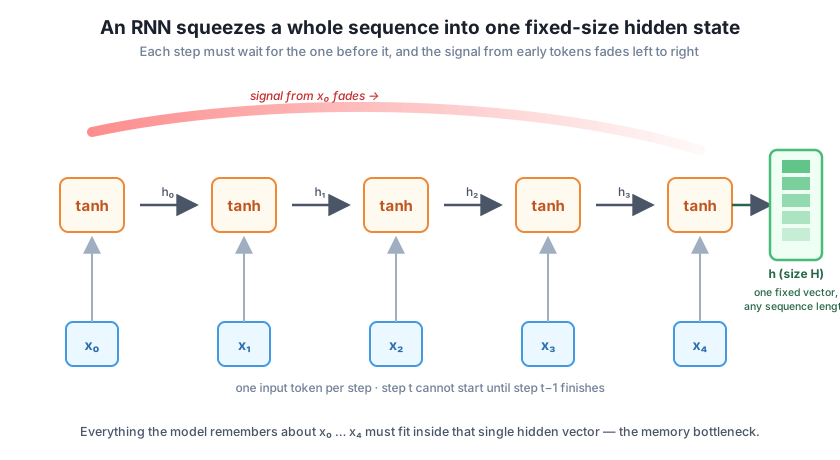
Hold those three measurements in mind, because the rest of this course is essentially their cure. The mechanism you’ll build next — attention — throws out the recurrent chain entirely. Instead of passing a single hidden state hand to hand down the sequence, attention lets every position look directly at every other position, in one parallel step.

That single change addresses all three limits at once. There’s no ordering dependency, so the whole sequence is processed in parallel rather than one step at a time (Limit 1). Every position keeps its own representation and can pull from any other, so there’s no single fixed vector forced to hold the entire past (Limit 2). And because any two positions are connected by exactly one hop — you saw that “longest path 1 hop” in the count above — the signal from a distant token arrives undiminished, and so does its gradient (Limit 3). The price is computing all $T^2$ pairwise interactions, but those are cheap, parallel, and, as you’ll see, the reason transformers scaled to models an RNN could never train.

In Lesson 2 you’ll build the core of that mechanism as a content-based weighted lookup: each position forms a query, compares it against every other position’s key, and pulls a weighted blend of their values. Everything starts there.

Practice Exercises#

Try these before checking the hints. They reuse the RNN code from this lesson.

Exercise 1: Memory Doesn’t Grow With Length#

Confirm the bottleneck for yourself. Run rnn_forward on sequences of length 3, 50, and 500, and print the shape of the final hidden state each time. Verify all three are identical even though the inputs differ wildly in length.

# Your code here (reuse Wx, Wh, b, and rnn_forward from the first demo)

Exercise 2: Does a Bigger Recurrent Weight Slow the Decay?#

In the decay experiment Wh was scaled by 0.35. Re-run the perturbation experiment with the scale set to 0.35, 0.55, and 0.75, and compare the influence at d = 20. Does a larger recurrent weight let the early signal travel farther?

# Your code here: wrap the decay experiment in a loop over the Wh scale

Exercise 3: Perturb a Late Token Instead#

The lesson changed the first token and watched its influence fade. Instead, perturb the last token x[T-1] and measure the difference at h_{T-1}. Explain in a comment why this influence is large even though the early-token influence was tiny.

# Your code here: perturb xs[T-1] instead of xs[0], compare h at the final step

Summary#

You built a real recurrent network in NumPy and watched it run into the exact walls that motivated the transformer. Let’s review.

Key Concepts#

How an RNN Reads

• Processes a sequence one step at a time: $h_t = \tanh(W_x x_t + W_h h_{t-1} + b)$
• The hidden state $h_t$ is the model’s entire memory of everything read so far

The Three Limits

• Sequential computation — step $t$ needs $h_{t-1}$, so the sequence can’t be processed in parallel; a length-$T$ sequence is $T$ ordered steps
• Fixed-size memory bottleneck — any-length history is crushed into one vector; our RNN produced shape (16,) for sequences of length 5 and 40 alike
• Fading long-range signal — a change to x_0 moved the hidden state by norm 2.74 at its own step but only ~1e-6 thirty steps later, a six-order-of-magnitude decay; the same shrinkage hits the gradient (the vanishing-gradient problem)

The Fix, Previewed

• Attention lets every position look at every other position in parallel: no ordering (fixes Limit 1), no single shared memory vector (fixes Limit 2), and a one-hop path between any two tokens (fixes Limit 3)

Why This Matters#

Recurrence was the state of the art in sequence modeling for years, and its limits weren’t obvious until people tried to scale it. Sequential processing capped how fast you could train on long text; the fixed hidden state capped how much context a model could truly use; and vanishing signal capped how far back a dependency could reach. Every one of those ceilings is a direct consequence of the single-vector, step-by-step design you just measured.

The transformer didn’t tweak the RNN — it replaced the recurrent chain with something that has none of those ceilings. Understanding why is what makes the coming lessons click rather than feel arbitrary. When you build attention next and see it compare all positions at once, you’ll recognize it immediately as the answer to the three numbers you just printed.

Continue Building Your Skills#

You now have a concrete, measured feel for what recurrence gives up: parallelism, unbounded memory, and long-range reach, all sacrificed to that single hand-me-down hidden state. In the next lesson you’ll build the mechanism that reclaims all three at once. You’ll implement attention as a content-based weighted lookup — each position will form a query, score it against every other position’s key with a dot product, turn those scores into weights with a softmax, and read out a weighted blend of value vectors. It’s the single idea the entire rest of this course rests on, and after watching an RNN’s memory fade to nothing, you’ll appreciate exactly why it changed everything.