Lesson 2 - The Attention Idea: Weighted Lookup

Welcome to The Attention Idea#

In the last lesson you saw the RNN bottleneck: a recurrent model has to cram everything it has read so far into one fixed-size hidden state, and by the time the lamp keeper’s story reaches “the boats come home when the lantern glows,” the early words have been squeezed almost out of memory. This lesson introduces the mechanism that removes that bottleneck entirely and powers every transformer you will build in this course: attention.

The whole idea fits in one sentence. Attention is a soft lookup: given a query, it compares that query against every key, turns the similarities into weights that sum to 1, and returns a weighted average of the values. Nothing is retrieved exactly; everything is blended by relevance. Get this one picture and the rest of the course is bookkeeping on top of it.

By the end of this lesson, you will be able to:

• Explain the difference between a hard dictionary lookup and a soft, content-based lookup
• Describe the three roles in attention: query, keys, and values
• Compute similarities with a dot product and turn them into weights with a stable softmax
• Return a weighted average of value vectors and confirm the weights sum to 1
• Show that a sharp query behaves like a near-hard lookup while an in-between query blends values

You need only NumPy and the softmax from Lesson 1. There are no learned parameters and no training here; this lesson is pure mechanism. Let’s begin.

From a Hard Lookup to a Soft One#

You already know one kind of lookup: a Python dictionary. You hand it a key, it finds the exact matching entry, and it returns that one value. Miss the key by a single character and you get nothing.

memory = {"dusk": 10, "fog": 20, "boat": 30}
print(memory["fog"])   # exact key -> exactly one value
# 20

That is a hard lookup. It is all-or-nothing: one key selected, everyone else ignored. It also cannot answer a fuzzy question. If your query is “sort of like fog, a little like dusk,” a dictionary has no way to blend the two.

Attention replaces this with a soft lookup. Instead of demanding an exact key match, it measures how similar the query is to every key, converts those similarities into a set of weights that sum to 1, and returns a weighted average of the values. A key that matches well gets a large weight; a key that matches poorly gets a small one; and the answer is a blend, weighted by relevance.

This is exactly the escape from the RNN bottleneck. In an RNN, position 12 can only see the past through one compressed hidden vector. With attention, position 12 issues a query and pulls content directly from every other position, as much or as little from each as their keys deserve. No information has to survive a long chain of hidden states.

The Three Roles: Query, Keys, Values#

Every attention computation has three cast members. Keeping them straight is most of the battle.

• Query (q): what the current position is looking for. One vector.
• Keys (K): a label for each item in memory, the thing a query is matched against. One vector per item.
• Values (V): the actual content returned for each item. One vector per item.

The keys and values come in matched pairs, item by item: key i is the searchable label for value i. The query never looks at the values directly. It matches against the keys to decide the weights, and those weights are then applied to the values. Separating “what you match on” (keys) from “what you return” (values) is what gives attention its flexibility.

In this lesson we use raw vectors as query, keys, and values. There are no learned projections yet; a query is just a vector, a key is just a vector, a value is just a vector. In Lesson 4 you will learn to produce q, k, and v from the same input with learned weight matrices, which is what makes attention trainable. For now we hand-set them so the mechanism is completely visible.

Step 1: Measure Similarity With a Dot Product#

How similar are two vectors? The simplest useful answer is the dot product. For a query $q$ and a key $k$, the score is

The dot product is large and positive when the two vectors point the same way, near zero when they are unrelated (orthogonal), and negative when they point in opposite directions. To score the query against every key at once, we stack the keys into a matrix $K$ of shape (number of keys, dimension) and compute $q K^\top$, giving one score per key.

Let’s set up a tiny toy memory. Four keys, each a simple 4-dimensional one-hot vector so the matching is easy to reason about, and four value vectors that carry the content each slot returns.

import numpy as np

np.random.seed(42)

# Four keys: searchable labels (one-hot so matches are easy to read)
keys = np.array([
    [1.0, 0.0, 0.0, 0.0],   # key 0
    [0.0, 1.0, 0.0, 0.0],   # key 1
    [0.0, 0.0, 1.0, 0.0],   # key 2
    [0.0, 0.0, 0.0, 1.0],   # key 3
])

# Four values: the content returned if a slot is selected
values = np.array([
    [10.0,  0.0],   # value 0
    [ 0.0, 10.0],   # value 1
    [ 5.0,  5.0],   # value 2
    [-5.0, -5.0],   # value 3
])

# A query that points strongly at key 0
q = np.array([3.0, 0.0, 0.0, 0.0])

scores = q @ keys.T          # dot product with every key -> (4,)
print("keys shape  :", keys.shape)
print("values shape:", values.shape)
print("scores      :", scores)

keys shape  : (4, 4)
values shape: (4, 2)
scores      : [3. 0. 0. 0.]

The query lines up with key 0 (score 3) and is orthogonal to the other three keys (score 0). Those raw scores are not yet weights: they do not sum to 1 and one of them could easily be negative. Turning them into a proper set of weights is the next step.

Step 2: Softmax the Scores Into Weights#

We want weights that are all positive and sum to 1, so the result is a genuine weighted average and a larger score always earns a larger weight. That is exactly what softmax does. For a vector of scores $s$,

We use the numerically stable form from Lesson 1: subtract the row maximum before exponentiating. This changes none of the weights (the constant cancels top and bottom) but keeps exp from overflowing on large scores.

def softmax(x, axis=-1):
    x = x - x.max(axis=axis, keepdims=True)   # stable: subtract the max
    e = np.exp(x)
    return e / e.sum(axis=axis, keepdims=True)

weights = softmax(scores)
print("weights:", np.round(weights, 4))
print("sum    :", weights.sum())

weights: [0.87   0.0433 0.0433 0.0433]
sum    : 1.0

The scores [3, 0, 0, 0] became weights [0.870, 0.043, 0.043, 0.043], and they sum to exactly 1. Key 0, the strong match, claims most of the weight, while the three unrelated keys each keep a small share. Notice that softmax never sends a weight fully to zero; even an orthogonal key retains a sliver. That is the “soft” in soft lookup, and it is what will let gradients flow once we start training.

Step 3: Return the Weighted Average of Values#

Now use the weights to blend the values. Each value is scaled by its key’s weight, and the scaled values are summed. With weights $w$ and value matrix $V$, the output is

out = weights @ values       # weighted average -> (2,)
print("blended output:", np.round(out, 4))

blended output: [8.7005 0.4332]

Read the result against the values. Value 0 is [10, 0] and it holds weight 0.870, so the output leans hard toward it: [8.70, 0.43] is almost [10, 0], pulled slightly by the small contributions of the other three values. The query asked for “key 0,” and it got back mostly value 0, blended with a faint trace of everything else. This is a near-hard lookup: soft in principle, but so concentrated it behaves almost like the dictionary we started with.

A Query Between Two Keys Blends Them#

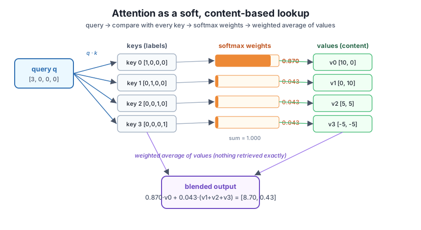
The near-hard case is only half the story. The real power of a soft lookup shows up when the query does not match any single key cleanly. Point the query halfway between key 0 and key 1 and watch what happens.

import numpy as np

np.random.seed(42)

keys = np.array([
    [1.0, 0.0, 0.0, 0.0],
    [0.0, 1.0, 0.0, 0.0],
    [0.0, 0.0, 1.0, 0.0],
    [0.0, 0.0, 0.0, 1.0],
])
values = np.array([
    [10.0,  0.0],
    [ 0.0, 10.0],
    [ 5.0,  5.0],
    [-5.0, -5.0],
])

def softmax(x, axis=-1):
    x = x - x.max(axis=axis, keepdims=True)
    e = np.exp(x)
    return e / e.sum(axis=axis, keepdims=True)

q = np.array([2.0, 2.0, 0.0, 0.0])   # points equally at key 0 and key 1

scores  = q @ keys.T
weights = softmax(scores)
out     = weights @ values

print("scores :", scores)
print("weights:", np.round(weights, 4), "sum =", round(float(weights.sum()), 6))
print("blend  :", np.round(out, 4))

scores : [2. 2. 0. 0.]
weights: [0.4404 0.4404 0.0596 0.0596] sum = 1.0
blend  : [4.404 4.404]

Now the query matches key 0 and key 1 equally (score 2 each), so softmax splits the weight evenly between them: 0.440 and 0.440, with the two unrelated keys sharing the rest. The output [4.404, 4.404] is a genuine blend of value 0 [10, 0] and value 1 [0, 10], landing squarely between them. No dictionary could produce this answer, because it corresponds to no single key. The soft lookup interpolates across memory, and that ability to mix content by relevance is precisely what a hard lookup can never do.

Practice Exercises#

Try these before checking the hints. They reuse the keys, values, and softmax defined above.

Exercise 1: Sharpen the Near-Hard Lookup#

Replace the query with q = np.array([6.0, 0.0, 0.0, 0.0]), an even stronger match to key 0. Recompute the weights and the blended output, and describe how the weight on key 0 and the output change compared to the [3, 0, 0, 0] query.

# Your code here (reuse keys, values, softmax)

Exercise 2: Query the Middle Key#

Set q = np.array([0.0, 0.0, 3.0, 0.0]) so the query points at key 2, whose value is [5, 5]. Predict the blended output before you run it, then check whether it lands near [5, 5].

# Your code here

Exercise 3: Confirm It Is a Weighted Average#

For any query, the output must be a convex combination of the value rows, so every component of the output has to fall within the range of that component across all four values. Take the q = [2, 2, 0, 0] result and verify that each output component lies between the minimum and maximum of the corresponding value column.

# Your code here

Summary#

You met the single most important idea in the course. Attention is a soft, content-based lookup, and you built the whole mechanism in a few lines of NumPy with no learned parameters at all. Let’s review.

Key Concepts#

The Big Idea

• A hard lookup (a dictionary) returns exactly one value for an exact key
• Attention is a soft lookup: compare a query to every key, softmax the similarities into weights that sum to 1, and return a weighted average of the values
• This is the escape from the RNN bottleneck: a position pulls content directly from every other position instead of through one compressed hidden state

The Three Roles

• Query: what the current position is looking for (one vector)
• Keys: the searchable label for each item in memory
• Values: the content returned for each item; keys are for matching, values are for returning
• This lesson uses raw vectors as q, k, v; learned projections come in Lesson 4

The Three Steps

• Similarity: scores = q @ keys.T, the dot product of the query with every key
• Weights: softmax(scores), positive and summing to 1, using the stable max-subtraction form
• Blend: weights @ values, the weighted average of the value vectors

What the Numbers Showed

• A sharp query [3, 0, 0, 0] gave weights [0.870, 0.043, 0.043, 0.043] and output [8.70, 0.43] — a near-hard lookup
• An in-between query [2, 2, 0, 0] gave weights [0.440, 0.440, 0.060, 0.060] and output [4.404, 4.404] — a genuine blend of two values
• The weights always sum to 1, so the output is always a convex combination of the values

Why This Matters#

Every transformer in existence, and the tiny GPT you are building in this course, is a deep stack of exactly this operation. When a language model reads a sentence and figures out which earlier word a pronoun refers to, it is issuing a query, matching it against the keys of every previous word, and averaging their values by relevance, precisely the three steps you just ran by hand. There is no other magic hiding underneath.

Holding on to the soft-lookup picture will make everything ahead easier. Scaled dot-product attention, multiple heads, causal masking, and the full self-attention layer are all refinements of this one mechanism: compare a query to keys, weight by relevance, average the values. You now own the intuition that the rest of the course is built on.

Continue Building Your Skills#

You have the core idea in your hands: attention is a weighted average of values, chosen by how well a query matches each key. What you built here worked on a single query and a fixed toy memory with numbers small enough to eyeball. In Lesson 3 you will scale this up to the shape transformers actually use, computing scores for a whole sequence at once as the matrix product $Q K^\top$, and you will meet the crucial $\frac{1}{\sqrt{hs}}$ scaling factor that keeps those scores from growing so large that softmax collapses onto a single key. That is the step that turns today’s hand-set demo into the scaled dot-product attention at the heart of every transformer block you will build next.