Lesson 3 - Similarity, Scores & Softmax Weights

Welcome to Similarity, Scores & Softmax Weights#

In the previous lesson you built attention as a weighted lookup: each position pulls information from every other position by taking a weighted average of their value vectors. You supplied the weights by hand to see the mechanism work. This lesson replaces that hand-waving with real machinery. You will learn exactly how a query and a set of keys produce those weights: score every key with a dot product, then squeeze the scores into a clean probability distribution with softmax. Along the way you will meet the numerical-stability trick that keeps softmax from blowing up, and the temperature knob that controls how sharply attention focuses.

This is the beating heart of the tiny char-level GPT you are building. Every attention head in the model does exactly this: dot products, softmax, weighted average. Get it solid here in NumPy and the full scaled dot-product attention of Module 2 will feel like a small step rather than a leap.

By the end of this lesson, you will be able to:

• Explain why the dot product measures similarity between a query and a key, and how it relates to cosine similarity and vector length
• Turn a vector of raw scores into a probability distribution with softmax, and state its two defining properties
• Implement the numerically stable softmax (subtract the max before exp) and show why the naive version overflows
• Use temperature scaling to make an attention distribution sharper or softer, and preview why Module 2 divides scores by $\sqrt{hs}$

You should be comfortable with NumPy arrays, matrix and vector multiplication, and the weighted-average idea from Lesson 2. Let’s begin.

Scoring With the Dot Product#

Attention needs a number for every key that says “how well does this key match the query?” The simplest good answer is the dot product. For a query vector $q$ and a key vector $k$, both of length $hs$, the score is

Why does this measure similarity? Recall the geometric identity that connects the dot product to the angle $\theta$ between two vectors:

Two vectors that point the same way have $\cos\theta = 1$ and a large positive dot product. Vectors at right angles have $\cos\theta = 0$ and a dot product of zero. Vectors pointing in opposite directions give a negative dot product. So a bigger dot product means a better match — the query and key are aligned in the embedding space. That is precisely the signal attention wants: keys aligned with the query should receive more weight.

Notice the identity also has the two lengths in it. The dot product is cosine similarity scaled by both vector norms. A key that points exactly at the query but is very short can still score lower than a mediocre-but-long key. This length sensitivity is real and it matters later: as vectors grow (for example when the head size $hs$ is large), dot products grow too, which is the problem the $\sqrt{hs}$ scaling in Module 2 exists to fix.

Let’s make it concrete. We create one query and five candidate keys of head size hs = 4, then score every key against the query with a single matrix-vector product.

import numpy as np

np.random.seed(42)

hs = 4
query = np.random.randn(hs)        # (4,)
keys = np.random.randn(5, hs)      # (5, 4) -- five candidate positions

scores = keys @ query              # (5,) one dot product per key
print("query:", np.round(query, 4))
print("scores (dot products):", np.round(scores, 4))
# Output:
# query: [ 0.4967 -0.1383  0.6477  1.523 ]
# scores (dot products): [ 2.1077 -1.3177 -1.5889 -3.2856 -1.367 ]

The single expression keys @ query computes all five dot products at once: row $i$ of keys is dotted with query to give scores[i]. Key 0 scores a strong positive 2.1077; the other four are negative, meaning they point somewhat away from the query. Already you can see attention will favor key 0.

To confirm the dot product really is length-scaled cosine similarity, compute both and compare.

cos = (keys @ query) / (np.linalg.norm(keys, axis=1) * np.linalg.norm(query))
print("cosine sims:", np.round(cos, 4))
print("key norms:  ", np.round(np.linalg.norm(keys, axis=1), 4))
# Output:
# cosine sims: [ 0.6805 -0.7813 -0.3462 -0.9544 -0.3833]
# key norms:   [1.7868 0.9729 2.6478 1.9859 2.0576]

Key 0 has cosine similarity 0.6805, the highest, and its raw dot-product score is the highest too. But look at keys 1 and 4: key 1 is more anti-aligned by cosine (-0.7813 versus -0.3833), yet their raw scores are nearly tied (-1.3177 versus -1.367). The reason is length: key 1 is short (norm 0.9729) while key 4 is long (norm 2.0576), and the norms drag the raw scores toward each other. That is length sensitivity in action, and it is exactly why unscaled dot products can behave unexpectedly.

From Scores to Weights: Softmax#

Raw scores are not yet usable as attention weights. Weights need to be non-negative (you cannot pull a negative amount of a value vector) and they need to sum to 1 (so the result is a genuine weighted average, not an arbitrary rescaling). The scores above are neither — most are negative and they sum to nothing in particular. Softmax is the function that fixes both problems at once. For a score vector $s$ it is defined as

Exponentiating makes every entry positive; dividing by the sum of all the exponentials forces the whole vector to add up to 1. The result is a probability distribution over the keys. And because exp is monotonic and grows fast, a score that is a little larger than the rest becomes a weight that is a lot larger — softmax gently exaggerates the winner, which is what we want when a query strongly matches one key.

Here is the naive definition, applied to our five scores.

def softmax_naive(s):
    e = np.exp(s)
    return e / e.sum()

weights = softmax_naive(scores)
print("weights:", np.round(weights, 4))
print("sum:", round(float(weights.sum()), 10))
print("argmax key:", int(np.argmax(weights)))
# Output:
# weights: [0.915  0.0298 0.0227 0.0042 0.0283]
# sum: 1.0
# argmax key: 0

The scores [2.11, -1.32, -1.59, -3.29, -1.37] became weights [0.915, 0.030, 0.023, 0.004, 0.028]. They are all positive, they sum to exactly 1.0, and key 0 — the best match — carries 0.915 of the total weight. If you fed these into the Lesson 2 lookup, the output would be almost entirely key 0’s value vector, with tiny contributions from the rest. That is content-based retrieval, computed for real.

Why the Naive Softmax Is Dangerous#

The naive softmax worked fine above because the scores were small. But exp grows explosively, and real attention scores can be large — especially before the $\sqrt{hs}$ scaling, or deep in a network where activations drift upward. Watch what happens with three larger scores.

big = np.array([1000.0, 1001.0, 1002.0])

e = np.exp(big)
print("exp(big):", e)
print("naive softmax:", e / e.sum())
# Output:
# exp(big): [inf inf inf]
# naive softmax: [nan nan nan]

exp(1000) is about $10^{434}$, far beyond the largest number a 64-bit float can hold (around $1.8 \times 10^{308}$), so it overflows to inf. Dividing inf by inf gives nan, and the NaNs then poison everything downstream — every weight, the weighted average, the loss, the gradients. A single overflow anywhere in a forward pass can silently destroy an entire training run.

The fix is a small algebraic trick. Softmax is shift-invariant: subtracting any constant $c$ from every score leaves the result unchanged, because the constant factors out of the ratio and cancels:

So we are free to choose $c$. The stable choice is $c = \max_j s_j$, the largest score. After subtracting the max, the biggest exponent becomes $e^0 = 1$ and every other exponent is between 0 and 1 — no overflow is possible, ever.

def softmax(s):
    s = s - np.max(s)          # shift so the largest score is 0
    e = np.exp(s)
    return e / e.sum()

print("stable softmax:", np.round(softmax(big), 6))
# Output:
# stable softmax: [0.090031 0.244728 0.665241]

No warnings, no NaNs, a clean distribution. And because the scores [1000, 1001, 1002] differ from [0, 1, 2] only by a constant shift of 1000, shift-invariance guarantees they must give the same weights — and they do: softmax([0, 1, 2]) is also [0.090031, 0.244728, 0.665241]. This softmax — subtract the max, exponentiate, normalize — is the exact function every attention head in your GPT will use. From here on, “softmax” means this stable version.

Temperature: Sharper or Softer Attention#

Softmax has a built-in focus knob. If you multiply or divide the scores by a constant before the softmax, you change how peaked the resulting distribution is, without changing which key ranks highest. Written with a temperature $\tau$, the scaled softmax is

A large $\tau$ (dividing by a big number) shrinks the gaps between scores, so the weights spread out toward uniform — softer, less decisive attention. A small $\tau$ (or multiplying the scores up) stretches the gaps, so the largest score runs away with almost all the weight — sharper, more decisive attention. Let’s see all three on our original five scores.

def softmax(s):
    s = s - np.max(s)
    e = np.exp(s)
    return e / e.sum()

for label, scaled in [("softer  (scores / 4)", scores / 4),
                      ("base    (scores    )", scores),
                      ("sharper (scores * 4)", scores * 4)]:
    w = softmax(scaled)
    print(f"{label}: {np.round(w, 4)}  max={w.max():.4f}")
# Output:
# softer  (scores / 4): [0.3999 0.1698 0.1587 0.1038 0.1678]  max=0.3999
# base    (scores    ): [0.915  0.0298 0.0227 0.0042 0.0283]  max=0.9150
# sharper (scores * 4): [1.     0.     0.     0.     0.    ]  max=1.0000

Same five scores, three very different distributions. Dividing by 4 flattens the weights toward uniform — key 0 still wins but only holds 0.40, and the other keys get a real say. Multiplying by 4 does the opposite: key 0 grabs essentially all the weight (0.999998, printed as 1.0000) and the rest collapse to near zero. The base case sits in between at 0.915.

You can put a single number on “how peaked” each distribution is with its entropy, $-\sum_i w_i \log w_i$: high entropy means spread out, low entropy means concentrated.

def entropy(p):
    return -np.sum(p * np.log(p + 1e-12))

print("entropy softer :", round(float(entropy(softmax(scores / 4))), 4))
print("entropy base   :", round(float(entropy(softmax(scores))), 4))
print("entropy sharper:", round(float(entropy(softmax(scores * 4))), 4))
# Output:
# entropy softer : 1.4944
# entropy base   : 0.3956
# entropy sharper: 0.0

The numbers confirm the picture: entropy falls from 1.4944 (softer) to 0.3956 (base) to 0.0000 (sharper, a winner-take-all distribution). Scaling scores up sharpens attention; scaling them down softens it.

This is not a curiosity — it is why the real formula divides. In Module 2 the attention scores are $QK^\top / \sqrt{hs}$, and that division by $\sqrt{hs}$ is a temperature. As explained earlier, dot products grow with vector length, so with a large head size $hs$ the raw scores $QK^\top$ become large, softmax saturates into a near one-hot spike (like our scores * 4 case), and gradients through that spike nearly vanish. Dividing by $\sqrt{hs}$ is the temperature that counteracts exactly that growth, keeping the distribution in a trainable middle range. You will derive the $\sqrt{hs}$ choice properly next module; for now, just hold onto the mechanism: scaling before softmax controls focus.

Putting It Together#

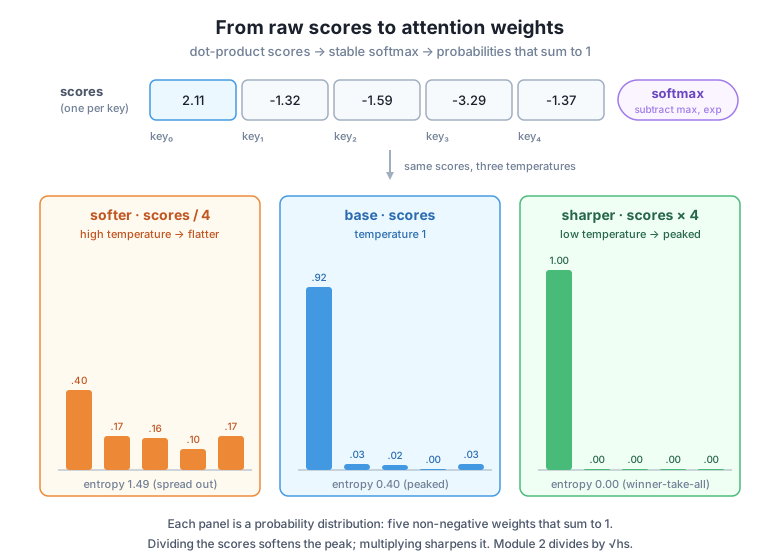
Here is the whole pipeline in one runnable block — score, stabilize, normalize, and scale — the exact operations one attention head performs. Run it twice; because everything is seeded, the output is identical every time.

import numpy as np

np.random.seed(42)

def softmax(s, axis=-1):
    s = s - s.max(axis=axis, keepdims=True)   # numerically stable
    e = np.exp(s)
    return e / e.sum(axis=axis, keepdims=True)

# 1. A query and five candidate keys, head size 4
hs = 4
query = np.random.randn(hs)
keys = np.random.randn(5, hs)

# 2. Dot-product similarity: one score per key
scores = keys @ query
print("scores :", np.round(scores, 4))

# 3. Softmax turns scores into attention weights
weights = softmax(scores)
print("weights:", np.round(weights, 4))
print("sum    :", round(float(weights.sum()), 6))
# Output:
# scores : [ 2.1077 -1.3177 -1.5889 -3.2856 -1.367 ]
# weights: [0.915  0.0298 0.0227 0.0042 0.0283]
# sum    : 1.0

Three lines of real math — a dot product, a stable softmax, a normalized distribution — and you have content-based attention weights. In Module 2 the query and keys will come from learnable projections of the input, the scores will be divided by $\sqrt{hs}$, and everything will run in batches of shape (B, T, T), but the core you just built does not change.

Practice Exercises#

Try these before checking the hints. They reuse the softmax, query, keys, and scores from the runnable block above.

Exercise 1: Prove Shift-Invariance Numerically#

The lesson claimed that adding any constant to every score leaves the softmax unchanged. Verify it: add 100 to all five scores, run the stable softmax on the shifted scores, and confirm the weights match the originals.

# Your code here: shift scores by +100 and compare softmax outputs

Exercise 2: Find the Temperature That Halves the Peak#

The base distribution puts 0.915 on key 0. Divide the scores by a temperature and find, by trying a few values, a $\tau$ that brings key 0’s weight down to roughly 0.5. Print the weight on key 0 for tau in [1, 2, 3, 4].

# Your code here: loop over tau values, print softmax(scores / tau)[0]

Exercise 3: Make the Naive Softmax Fail, Then Fix It#

Reproduce the overflow yourself. Build a score vector with one large value, np.array([50.0, 800.0, 20.0]), and confirm that a naive exp(s) / exp(s).sum() gives nan while the stable softmax gives a clean distribution.

# Your code here: compare naive vs stable softmax on [50.0, 800.0, 20.0]

Summary#

You built the two operations that turn vectors into attention weights: dot-product scoring and softmax normalization, plus the temperature knob that controls focus. Let’s review.

Key Concepts#

Dot-Product Similarity

• The score for a key is the dot product with the query: $q \cdot k = \sum_d q_d k_d$
• Geometrically $q \cdot k = \lVert q \rVert \lVert k \rVert \cos\theta$, so a bigger dot product means better alignment — the query and key point the same way
• The dot product is cosine similarity scaled by both vector lengths, so long keys score higher for the same direction; this length growth is what $\sqrt{hs}$ will later correct

Softmax

• $\text{softmax}(s)_i = e^{s_i} / \sum_j e^{s_j}$ turns any score vector into a probability distribution: every weight positive, all weights summing to 1
• It is a smooth, differentiable soft argmax: the top score gets most of the weight but every key keeps a little, so gradients can flow

Numerical Stability

• exp of a large score overflows to inf, and inf / inf is nan that poisons the whole forward pass
• Softmax is shift-invariant, so subtracting the max score before exp changes nothing mathematically but guarantees no overflow: s = s - s.max() first, always

Temperature Scaling

• Scaling scores before softmax controls peakiness: dividing (high temperature) softens toward uniform, multiplying (low temperature) sharpens toward one-hot
• On our scores, /4 gave entropy 1.49, base gave 0.40, *4 gave 0.00
• Module 2’s $QK^\top / \sqrt{hs}$ is exactly this temperature, chosen to counteract the growth of dot products with head size

Why This Matters#

Every attention head in every transformer — including the tiny char-level GPT you are building — runs this exact pipeline millions of times: dot products to score, softmax to normalize, weighted average to retrieve. When you understand that the weights come from alignment in embedding space, that the max-subtraction is not optional cleanliness but the difference between a working model and a screen full of NaNs, and that a single scaling constant decides whether attention is razor-focused or blurry, you can read and debug real attention code with confidence. A model that “attends to everything equally” or “collapses onto one token” is almost always a temperature problem, and now you know where to look.

Continue Building Your Skills#

You can now take a query and a set of keys and produce honest attention weights — non-negative, summing to one, sharpened or softened on demand, and safe from overflow. But so far the queries, keys, and values have been handed to you as raw vectors. In the next lesson, Learnable Projections: Query, Key & Value, you will see where they actually come from: three weight matrices that project each input embedding into a query, a key, and a value. That is the step that makes attention learnable — the model discovers, through training, what to look for and what to retrieve — and it turns the fixed scoring you built here into the trainable attention head at the center of the transformer.