Lesson 4 - From Lookup to Learned Attention

Welcome to From Lookup to Learned Attention#

In the last two lessons you built attention as a content-based lookup: every position produced a query, compared it against every key by dot product, turned those scores into weights with softmax, and read back a weighted average of the values. It worked, and it was fully differentiable. But there was a quiet limitation hiding in it: you used the raw input vectors themselves as the query, the key, and the value. That choice silently fixes what “similar” means and what “content” gets returned. The model had no say in it.

This lesson removes that limitation. Instead of feeding the input straight into the attention math, you first project it through three learned weight matrices, $W_q, W_k, W_v$, into three separate spaces: a query space, a key space, and a value space. Similarity is then measured in the learned query/key space, and the content that comes back lives in the learned value space. Because those matrices are parameters, the network can learn, from data, which relationships are worth attending to. This is the exact attention head your mini-GPT will use, and the mechanism Module 2 formalizes.

By the end of this lesson, you will be able to:

• Explain why using raw input vectors as query, key, and value is a limitation
• Describe the role and shape of the three projection matrices $W_q, W_k, W_v$
• Trace the shapes through the parameterized attention head: X, Q/K/V, scores, weights, out
• Implement the projected self-attention forward pass in pure NumPy
• Show that changing a projection (Wq) changes which positions attend to which

You should be comfortable with the dot-product-and-softmax lookup from Lessons 2 and 3, and with NumPy matrix multiplication and broadcasting. There is no training in this lesson, just the parameterized forward pass and its shapes. Let’s begin.

The Limitation of a Raw Lookup#

Recall the lookup you built. Given a stack of token vectors $X$ of shape (B, T, C), you compared each token against every other by taking dot products of the vectors themselves, softmaxed the scores into weights, and averaged the same vectors as the returned content. In pseudo-form it was softmax(X @ X.transpose) @ X.

Look closely at what that fixes. The input vector plays three different roles at once: it is the query that goes looking, the key that gets matched against, and the value that gets returned. But those are genuinely different jobs. What makes a good search query is not necessarily what makes a good thing to be searched, and neither is necessarily the information you want to carry forward. By forcing one vector to do all three, you hard-code a single notion of similarity, the raw dot product in the input space, and a single notion of content, the input itself.

Concretely, suppose a token wants to attend to “the noun three positions back” but ignore “the token that looks most similar to me.” A raw dot-product lookup cannot express that: similarity is whatever the input geometry happens to give you. There is no knob to turn. We want a knob, and we want the network to learn where to set it.

The Fix: Project Into Three Learned Spaces#

The fix is small to write and large in consequence. Before computing any similarity, pass the input through three separate learned linear maps:

Each of $W_q, W_k, W_v$ is a weight matrix of shape (C, hs), where C is the model width (n_embd, 64 in our config) and hs is the head size (16). Multiplying the input (B, T, C) by a (C, hs) matrix produces (B, T, hs): every token is re-expressed as an hs-dimensional vector in a new, learned space.

• $W_q$ builds the query: what this position is looking for.
• $W_k$ builds the key: how this position advertises itself to others.
• $W_v$ builds the value: what this position hands over when it is attended to.

Now the dot product $Q K^\top$ measures similarity in the learned query/key space rather than in the raw input space, and the returned average $\text{weights} \cdot V$ lives in the learned value space. The three matrices are parameters, so gradient descent (later in the course) will tune them so that the right positions match and the right content flows. That is the entire idea: we replaced a fixed similarity with a learned one.

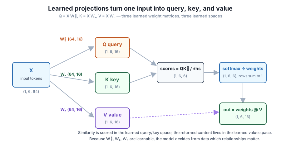
Everything downstream, the scaled dot product, the softmax, the weighted average of values, is exactly the lookup you already know. The only change is that Q, K, and V are now learned projections of the input rather than the input itself.

The Shapes, End to End#

Keeping shapes straight is the fastest way to understand a new layer, so let us name every one. With batch B, sequence length T, model width C, and head size hs:

• X is (B, T, C): the input, one C-dimensional vector per token.
• Wq, Wk, Wv are each (C, hs): the learned projection matrices.
• Q, K, V are each (B, T, hs): the projected query, key, and value.
• scores = Q @ K.transpose(0, 2, 1) / sqrt(hs) is (B, T, T): how much each position matches every other.
• weights = softmax(scores) is (B, T, T): the same, normalized so each row sums to 1.
• out = weights @ V is (B, T, hs): the attended output, one hs-vector per token.

The (B, T, T) shape of scores and weights is the giveaway that this is attention: it is a full table of every position against every position. The division by $\sqrt{hs}$ is the scaling from the brief that keeps the dot products from growing too large as hs increases; Module 2 explains exactly why. For now, notice that the input arrived as (B, T, C) and the output leaves as (B, T, hs), so a head reshapes the model width from C down to hs while mixing information across positions.

Building the Parameterized Forward in NumPy#

Here is the parameterized self-attention forward pass, in pure NumPy. This is the reference self_attention you will reuse for the rest of the course; here we run it non-causal (every position may attend to every other) because masking comes later, in Module 6.

import numpy as np

def softmax(x, axis=-1):
    x = x - x.max(axis=axis, keepdims=True)   # subtract row max for stability
    e = np.exp(x)
    return e / e.sum(axis=axis, keepdims=True)

def self_attention(X, Wq, Wk, Wv, causal=False):
    # X: (B, T, C);  Wq/Wk/Wv: (C, hs)
    Q, K, V = X @ Wq, X @ Wk, X @ Wv                  # each (B, T, hs)
    hs = Q.shape[-1]
    scores = Q @ K.transpose(0, 2, 1) / np.sqrt(hs)   # (B, T, T)
    if causal:
        T = scores.shape[1]
        mask = np.triu(np.ones((T, T), dtype=bool), k=1)
        scores = np.where(mask, -1e9, scores)
    weights = softmax(scores, axis=-1)                # (B, T, T)
    return weights @ V, weights                       # out: (B, T, hs)

Now feed it a small random input and three random projections, and print the shape at every stage. We use a fixed seed so the run is fully reproducible, and a modest projection scale (* 0.25) so the attention weights come out clearly differentiated rather than nearly uniform.

rng = np.random.default_rng(42)
B, T, C, hs = 1, 6, 64, 16
X = rng.standard_normal((B, T, C))          # (1, 6, 64): 6 tokens, width 64

Wq = rng.standard_normal((C, hs)) * 0.25    # (64, 16)
Wk = rng.standard_normal((C, hs)) * 0.25    # (64, 16)
Wv = rng.standard_normal((C, hs)) * 0.25    # (64, 16)

Q, K, V = X @ Wq, X @ Wk, X @ Wv
print("X:", X.shape, " Wq/Wk/Wv:", Wq.shape)
print("Q:", Q.shape, " K:", K.shape, " V:", V.shape)

out, weights = self_attention(X, Wq, Wk, Wv)
print("scores/weights:", weights.shape, " out:", out.shape)
print("weights row sums:", np.round(weights.sum(-1), 6))
print("weights[0]:")
print(np.round(weights[0], 3))
print("each position attends most to:", weights[0].argmax(-1))

X: (1, 6, 64)  Wq/Wk/Wv: (64, 16)
Q: (1, 6, 16)  K: (1, 6, 16)  V: (1, 6, 16)
scores/weights: (1, 6, 6)  out: (1, 6, 16)
weights row sums: [[1. 1. 1. 1. 1. 1.]]
weights[0]:
[[0.    0.004 0.003 0.988 0.    0.005]
 [0.028 0.138 0.087 0.002 0.203 0.541]
 [0.    0.002 0.001 0.003 0.002 0.993]
 [0.989 0.    0.    0.007 0.002 0.002]
 [0.    0.001 0.024 0.009 0.042 0.923]
 [0.032 0.004 0.    0.511 0.009 0.445]]
each position attends most to: [3 5 5 0 5 3]

Read that off against the shape list: X came in at (1, 6, 64), the three projections mapped it to Q, K, V at (1, 6, 16), the query-key comparison produced a (1, 6, 6) attention table, and the output left at (1, 6, 16). Every row of weights sums to 1, exactly as softmax over the last axis guarantees, so each token’s output is an honest weighted average of the six value vectors. The argmax line reads as: position 0 attends most to position 3, positions 1 and 4 to position 5, and so on. Nothing was trained; this pattern is simply the one these particular random projections happen to induce.

The Projections Control What Attention Does#

The claim of this lesson is that the projections, not the input, decide what attention does. Here is the experiment that shows it. Keep X, Wk, and Wv exactly as before, and change only Wq, the query projection. If the projections really are the knob, the attention pattern should change even though the input is untouched.

rng2 = np.random.default_rng(1)
Wq2 = rng2.standard_normal((C, hs)) * 0.25   # a different learned query projection

out2, weights2 = self_attention(X, Wq2, Wk, Wv)
print("weights2[0]:")
print(np.round(weights2[0], 3))
print("each position attends most to:", weights2[0].argmax(-1))
print("attention pattern changed?", not np.allclose(weights, weights2))
print("out2:", out2.shape)

weights2[0]:
[[0.018 0.004 0.139 0.038 0.714 0.087]
 [0.961 0.026 0.002 0.002 0.009 0.   ]
 [0.53  0.001 0.461 0.    0.008 0.   ]
 [0.923 0.036 0.037 0.    0.004 0.   ]
 [0.052 0.002 0.081 0.677 0.17  0.018]
 [0.923 0.002 0.    0.071 0.002 0.001]]
each position attends most to: [4 0 0 0 3 0]

attention pattern changed? True
out2: (1, 6, 16)

The input never moved, yet the attention pattern is completely different. With the first query projection, the positions attended most to [3 5 5 0 5 3]; with the second, to [4 0 0 0 3 0]. Same tokens, same keys, same values, but a different learned query changed what every position looks for and therefore what content it pulls back. The output shape stayed (1, 6, 16), because the shapes are set by C and hs, not by the particular numbers in the weights.

That is the payoff. In this lesson the projections were random, so the pattern was arbitrary. Once the course reaches training, gradient descent will adjust $W_q, W_k, W_v$ so that the patterns are useful, so that a position learns to attend to the tokens that actually help predict the next character in the Lantern Bay corpus. The mechanism is already in your hands; only the learning is still to come.

Practice Exercises#

Try these before checking the hints. They reuse the softmax and self_attention functions and the variables defined above.

Exercise 1: Verify the Projection Shapes#

Change the head size to hs = 8 while keeping C = 64, rebuild Wq, Wk, Wv, and confirm that Q, K, V become (1, 6, 8), that weights stays (1, 6, 6), and that out becomes (1, 6, 8). Explain in a comment why weights did not change shape.

# Your code here: set hs = 8, remake the projections, print Q/K/V/weights/out shapes

Exercise 2: Confirm the Rows Are a Probability Distribution#

For the original weights (with hs = 16), verify two things numerically: every entry is between 0 and 1, and every row sums to 1. Print a single boolean for each check.

# Your code here: check the range and the row sums of weights

Exercise 3: Change Wk Instead of Wq#

Repeat the control experiment, but this time hold X, Wq, and Wv fixed and change only Wk, the key projection. Confirm the attention pattern changes, and explain in a comment why changing either side of the query-key dot product has the same kind of effect.

# Your code here: make a new Wk, run self_attention, compare argmax rows to the original

Summary#

You upgraded the fixed content-based lookup into a learnable attention head by inserting three projection matrices between the input and the attention math. Let’s review.

Key Concepts#

The Limitation

• Using the raw input vector as query, key, and value forces one vector to play three different roles and hard-codes a single notion of similarity
• There is no way for the model to learn what to look for

The Fix: Learned Projections

• Project the input into three separate learned spaces: $Q = X W_q$, $K = X W_k$, $V = X W_v$
• $W_q, W_k, W_v$ are each (C, hs) weight matrices and are the trainable parameters of a head
• Similarity is now computed in the learned query/key space; content is returned from the learned value space

The Shapes

• X: (B, T, C) → Q, K, V: (B, T, hs) → scores/weights: (B, T, T) → out: (B, T, hs)
• The (B, T, T) attention table is the signature of attention; each row is a probability distribution that sums to 1

Why It Matters in Practice

• The projections, not the input, control which positions attend to which: changing Wq alone rewired the whole pattern while X stayed fixed
• Training (later in the course) tunes $W_q, W_k, W_v$ so the patterns become useful for predicting the next character

Why This Matters#

This is the exact attention head that sits inside every transformer, from the tiny char-level GPT you are building to the largest language models in production. The single design decision you made in this lesson, project the input into separate query, key, and value spaces before comparing, is what turns attention from a fixed geometric operation into a trainable one. Everything else in the architecture, multiple heads, stacking layers, causal masking, is an elaboration on top of this one idea.

Understanding it as projections also pays off when you read real transformer code. When you see nn.Linear layers named q_proj, k_proj, and v_proj, you now know precisely what they are: the $W_q, W_k, W_v$ matrices you just implemented, mapping the model width C into a head size hs. And you know how to debug them, because you have already traced every shape from X to out by hand.

Continue Building Your Skills#

You now have a complete, parameterized attention head: an input projected into query, key, and value, compared in a learned space, and read back as a weighted average. What you have not done yet is put it to work on real text. In the next lesson, a guided project, you will take this exact self_attention forward pass and run it over the Lantern Bay corpus itself, encoding a slice of characters into vectors, projecting them, and inspecting the attention weights to see which characters each position leans on. It is the moment the abstract (B, T, hs) shapes become a concrete lookup over “the lamp keeper walks the shore,” and the last step before Module 2 derives the scaled dot-product attention you built here from first principles.