Lesson 5 - Guided Project: A Retrieval-Style Attention Layer

Welcome to the Guided Project#

Across this module you met the pieces of attention one at a time: why recurrence struggles on long sequences, how a content-based lookup pulls information from every position, how dot-product similarity and softmax turn raw scores into weights, and how learnable query, key, and value projections make the whole thing trainable. In this guided project you snap those pieces together into a single small attention layer that actually runs — the first working organ of the tiny char-level GPT you build across the rest of the course.

You will work over the course’s real corpus, the Lantern Bay passage, and do it in four short stages. Each stage runs in pure NumPy, is fully reproducible with np.random.seed(42), and prints real shapes and numbers so you can see the data flow with your own eyes. By the end you will have taken text all the way to an attention weight matrix — and you will notice something surprising about how repeated characters behave that motivates the very next module.

By the end of this project, you will be able to:

• Tokenize the Lantern Bay corpus at the character level and recover text with encode and decode
• Turn a slice of token ids into an embedded sequence tensor of shape (1, T, C)
• Run one learned self-attention layer with query/key/value projections and read off every intermediate shape
• Confirm that attention weight rows form a probability distribution (each row sums to 1)
• Interpret a real attention matrix, and explain why identical tokens attend identically before positions are added

This project assumes you have followed the earlier lessons in this module. You only need numpy installed (version 2.x is fine) and nothing else — no PyTorch, no GPU, no API key.

Stage 1: Tokenize the Corpus#

Everything the model ever sees is numbers, so the first job is turning text into integers. We use character-level tokenization: every distinct character in the corpus becomes one token id. The Lantern Bay corpus is a short original passage repeated to give a tiny model a low-entropy target to learn later. We build the vocabulary from its unique characters, then define encode (text to ids) and decode (ids back to text).

import numpy as np
import warnings
warnings.filterwarnings("ignore")

CORPUS = (
    "the lamp keeper walks the shore at dusk. "
    "the lamp keeper lights the lantern when the fog rolls in. "
    "the boats come home when the lantern glows. "
    "the boats wait outside the bay when the fog is thick. "
    "a small boat drifts near the rocks at dawn. "
    "the keeper rings the bell when a boat drifts near the rocks. "
    "the tide rises at dusk and falls at dawn. "
    "the gulls call over the bay when the tide is low. "
    "the keeper counts the boats and writes the count in a book. "
    "the lantern burns all night and rests at dawn. "
) * 20

chars = sorted(set(CORPUS))
vocab_size = len(chars)
stoi = {c: i for i, c in enumerate(chars)}
itos = {i: c for i, c in enumerate(chars)}
encode = lambda s: [stoi[c] for c in s]
decode = lambda ids: "".join(itos[i] for i in ids)
data = np.array(encode(CORPUS), dtype=np.int64)

print("vocab_size:", vocab_size)
print("len(data):", len(data))
print("first 12 ids:", data[:12].tolist())
print("decoded[:24]:", repr(decode(data[:24].tolist())))

vocab_size: 24
len(data): 10020
first 12 ids: [19, 9, 6, 0, 12, 2, 13, 16, 0, 11, 6, 6]
decoded[:24]: 'the lamp keeper walks th'

The vocabulary is exactly 24 characters: the 26 lowercase letters that appear, plus a space and a period — but only the letters the passage actually uses, which lands the count at 24. The full corpus encodes to 10020 token ids. The round trip works: ids [19, 9, 6, 0, ...] decode straight back to "the lamp keeper walks th", which is the start of the passage. That decode(encode(text)) == text property is the sanity check that our tokenizer is lossless.

Stage 2: Embed a Sequence#

Token ids are just labels — id 6 is not “greater than” id 2 in any meaningful way, so we cannot feed raw ids into matrix math. Instead each id indexes into an embedding table: a matrix of shape (vocab_size, C) where row i is the learnable vector for token i. Here C = 32 is the model width (the number of features per token). We take the first T = 12 characters of the corpus, look up each one’s embedding, and add a leading batch dimension so the result has the course’s canonical activation shape (B, T, C).

np.random.seed(42)
C = 32                 # model width (features per token)
T = 12                 # sequence length (a short slice)
embed_table = np.random.randn(vocab_size, C)   # (vocab_size, C)

ids = data[:T]                       # (T,) the first 12 token ids
X = embed_table[ids][None, :, :]     # (1, T, C) add the batch axis

print("ids:", ids.tolist())
print("chars:", [itos[i] for i in ids.tolist()])
print("embed_table.shape:", embed_table.shape)
print("X.shape:", X.shape)

ids: [19, 9, 6, 0, 12, 2, 13, 16, 0, 11, 6, 6]
chars: ['t', 'h', 'e', ' ', 'l', 'a', 'm', 'p', ' ', 'k', 'e', 'e']
embed_table.shape: (24, 32)
X.shape: (1, 12, 32)

The slice we embedded spells out t h e _ l a m p _ k e e (the space is shown as _ here), the opening of “the lamp keeper.” The fancy indexing embed_table[ids] gathers 12 rows into a (12, 32) array, and [None, :, :] prepends the batch dimension to give (1, 12, 32): one sequence, twelve positions, thirty-two features each. That is (B, T, C) with B = 1, T = 12, C = 32 — the exact layout every attention layer in this course expects.

Notice already that positions 2, 10, and 11 are all the character 'e', and positions 3 and 8 are both a space. Those repeated characters share the same embedding row, because the embedding depends only on the token id, not on where it sits. Hold that thought — it becomes the punchline of Stage 4.

Stage 3: Run One Learned Attention Layer#

Now the heart of the module. Self-attention projects each token’s embedding into three roles — a query (what am I looking for?), a key (what do I offer?), and a value (what will I hand over?) — using three learnable weight matrices Wq, Wk, Wv, each of shape (C, hs) where hs = 16 is the head size. It then scores every query against every key with a scaled dot product, softmaxes the scores into weights, and returns a weighted average of the values. This is the exact self_attention function the module derived; we run it non-causal (every position may look at every other) for this project.

def softmax(x, axis=-1):
    x = x - x.max(axis=axis, keepdims=True)   # stable: subtract row max
    e = np.exp(x)
    return e / e.sum(axis=axis, keepdims=True)

def self_attention(X, Wq, Wk, Wv, causal=False):
    # X: (B, T, C);  Wq/Wk/Wv: (C, hs)
    Q, K, V = X @ Wq, X @ Wk, X @ Wv                  # each (B, T, hs)
    hs = Q.shape[-1]
    scores = Q @ K.transpose(0, 2, 1) / np.sqrt(hs)   # (B, T, T)
    if causal:
        Tn = scores.shape[1]
        mask = np.triu(np.ones((Tn, Tn), dtype=bool), k=1)
        scores = np.where(mask, -1e9, scores)
    weights = softmax(scores, axis=-1)                # (B, T, T)
    out = weights @ V                                 # (B, T, hs)
    return out, weights, Q, K, V, scores

np.random.seed(42)
hs = 16
Wq = np.random.randn(C, hs) * 0.1
Wk = np.random.randn(C, hs) * 0.1
Wv = np.random.randn(C, hs) * 0.1

out, weights, Q, K, V, scores = self_attention(X, Wq, Wk, Wv, causal=False)

print("Q.shape:", Q.shape, "K.shape:", K.shape, "V.shape:", V.shape)
print("scores.shape:", scores.shape)
print("weights.shape:", weights.shape)
print("out.shape:", out.shape)
print("row sums:", np.round(weights[0].sum(axis=1), 6).tolist())

Q.shape: (1, 12, 16) K.shape: (1, 12, 16) V.shape: (1, 12, 16)
scores.shape: (1, 12, 12)
weights.shape: (1, 12, 12)
out.shape: (1, 12, 16)
row sums: [1.0, 1.0, 1.0, 1.0, 1.0, 1.0, 1.0, 1.0, 1.0, 1.0, 1.0, 1.0]

Every shape lands exactly where the conventions say it should. Projecting X of shape (1, 12, 32) through the (32, 16) weight matrices gives Q, K, and V, each (1, 12, 16). The scores Q K^\top / \sqrt{hs} compare all 12 queries against all 12 keys, producing the (1, 12, 12) grid, and softmax over the last axis turns each row into a probability distribution. The proof is the row sums: all twelve are exactly 1.0, so each query spreads a total attention weight of 1 across the keys. Finally weights @ V mixes the values into the output (1, 12, 16) — one refined vector per position, each a blend of the whole sequence.

The dimension of the scores matrix is worth pausing on. It is $\text{scores} = \frac{Q K^\top}{\sqrt{hs}}$, and the scaling by $\sqrt{hs}$ keeps the dot products from growing large as the head size increases, which would otherwise push softmax into near-one-hot saturation.

Stage 4: Inspect the Attention#

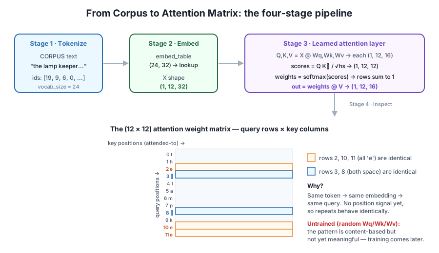
The weights matrix is the whole point of attention: row t tells you how much position t (the query) pulls from each other position (the keys). Let’s print it, rounded, alongside the tokens so we can read it like a table.

np.set_printoptions(precision=3, suppress=True, linewidth=200)
print("tokens:", [itos[i] for i in ids.tolist()])
print("attention weights (T x T):")
print(np.round(weights[0], 3))
print("argmax attended position per query row:", weights[0].argmax(axis=1).tolist())

tokens: ['t', 'h', 'e', ' ', 'l', 'a', 'm', 'p', ' ', 'k', 'e', 'e']
attention weights (T x T):
[[0.111 0.095 0.092 0.067 0.076 0.066 0.061 0.078 0.067 0.103 0.092 0.092]
 [0.092 0.085 0.083 0.069 0.1   0.072 0.087 0.087 0.069 0.09  0.083 0.083]
 [0.127 0.108 0.07  0.047 0.138 0.08  0.078 0.101 0.047 0.063 0.07  0.07 ]
 [0.061 0.074 0.059 0.1   0.102 0.085 0.103 0.084 0.1   0.114 0.059 0.059]
 [0.063 0.064 0.1   0.124 0.039 0.05  0.093 0.087 0.124 0.057 0.1   0.1  ]
 [0.067 0.085 0.086 0.075 0.087 0.091 0.079 0.089 0.075 0.091 0.086 0.086]
 [0.088 0.093 0.07  0.065 0.102 0.068 0.058 0.065 0.065 0.187 0.07  0.07 ]
 [0.048 0.08  0.078 0.067 0.116 0.095 0.135 0.104 0.067 0.053 0.078 0.078]
 [0.061 0.074 0.059 0.1   0.102 0.085 0.103 0.084 0.1   0.114 0.059 0.059]
 [0.077 0.077 0.088 0.083 0.073 0.083 0.081 0.107 0.083 0.074 0.088 0.088]
 [0.127 0.108 0.07  0.047 0.138 0.08  0.078 0.101 0.047 0.063 0.07  0.07 ]
 [0.127 0.108 0.07  0.047 0.138 0.08  0.078 0.101 0.047 0.063 0.07  0.07 ]]
argmax attended position per query row: [0, 4, 4, 9, 3, 9, 9, 6, 9, 7, 4, 4]

Read row 6 (the query at position 6, the character 'm'): its largest weight, 0.187, sits in column 9 (the 'k' of “keeper”), so this query attends most to that position. Every row is a full distribution — the values are all in a fairly narrow band around 1/12 ≈ 0.083 because the projections are small and untrained, so no single connection dominates hugely. That narrow spread is itself informative: untrained attention is close to a uniform average, and training is what will later sharpen these rows into the crisp, meaningful lookups you have read about.

Now the surprising part, and the reason this project exists. Look at the token list: positions 2, 10, and 11 are all 'e', and positions 3 and 8 are both a space. Compare their rows in the matrix — they are identical, not merely similar. Let’s prove it rather than eyeball it.

w = weights[0]
print("rows 2,10,11 (all 'e') identical:",
      np.allclose(w[2], w[10]) and np.allclose(w[10], w[11]))
print("rows 3,8 (both space) identical:", np.allclose(w[3], w[8]))
print("cols 2,10,11 identical:",
      np.allclose(w[:, 2], w[:, 10]) and np.allclose(w[:, 10], w[:, 11]))
print("cols 3,8 identical:", np.allclose(w[:, 3], w[:, 8]))

rows 2,10,11 (all 'e') identical: True
rows 3,8 (both space) identical: True
cols 2,10,11 identical: True
cols 3,8 identical: True

Repeated characters attend identically — and are attended to identically — because attention here is purely content-based. Position 2 and position 11 are both 'e', so they share the same embedding, so they produce the same query and the same key, so their rows (and their columns) come out exactly equal. The layer literally cannot tell the three 'e' positions apart. This is not a bug; it is the honest behavior of attention with no notion of order. A language model obviously must distinguish “the first e” from “the last e,” and the fix — positional encoding — is precisely what a later module adds.

You have now taken raw text all the way to a working attention layer and read its output. Run the whole script a second time: because every random draw is seeded with np.random.seed(42), you get byte-for-byte identical numbers. That reproducibility is what lets us verify every claim in this course by simply re-running the code.

Practice Exercises#

Try these before checking the hints. They reuse the CORPUS, encode, embed_table, and self_attention you built above.

Exercise 1: Embed a Different Slice#

Instead of the first 12 characters, embed the slice data[100:112]. Decode it to see the text, build X, and confirm its shape is still (1, 12, 32). Which characters in this slice repeat?

# Your code here: slice data[100:112], decode it, build X, print X.shape

Exercise 2: Turn On the Causal Mask#

Re-run self_attention with causal=True and print the weight matrix. Confirm that position 0’s row now has weight only in column 0, and that the whole matrix is lower-triangular (zeros above the diagonal).

# Your code here: call self_attention(X, Wq, Wk, Wv, causal=True)

Exercise 3: Break the Tie Between Repeated Characters#

Add a simple position signal so the three 'e' positions stop being identical: create a (T, C) matrix of small random “position embeddings” and add it to X before calling self_attention. Re-check whether rows 2, 10, and 11 are still equal.

# Your code here: pos = np.random.randn(T, C) * 0.1; X2 = X + pos[None, :, :]

Summary#

You assembled Module 1 into one runnable attention layer and drove real text through it, end to end, in pure NumPy. Let’s review what you built.

Key Concepts#

The Pipeline

• Tokenize: character-level encode/decode over the Lantern Bay corpus gives vocab_size = 24 and a 10020-token data array
• Embed: an (vocab_size, C) table maps each token id to a C = 32 vector; a T = 12 slice becomes X of shape (1, 12, 32) = (B, T, C)
• Attend: learnable Wq, Wk, Wv of shape (C, hs) with hs = 16 produce Q, K, V of (1, 12, 16), scores and weights of (1, 12, 12), and output of (1, 12, 16)
• Inspect: each weight row sums to 1 (a probability distribution over keys)

What the Matrix Revealed

• Untrained attention is close to a uniform average — no single connection dominates strongly
• Identical tokens (the three 'e's, the two spaces) produce identical rows and columns, because attention here is purely content-based with no positional signal
• The argmax per row shows which key each query prefers, but with random weights that preference is arbitrary — only the structure (rows sum to 1, repeats match) is guaranteed

Reproducibility

• Seeding every block with np.random.seed(42) makes the entire pipeline byte-for-byte repeatable, so every printed number can be verified by re-running

Why This Matters#

This tiny layer is the seed of the GPT you grow for the rest of the course. Everything you add later — multiple heads, a causal mask, position information, stacked blocks, and finally training — hangs on the (B, T, C) in, attention in the middle, (B, T, hs) out skeleton you just built. Because you assembled it from scratch, you now know exactly what each shape means and why the row sums must be 1, which is the kind of understanding that makes debugging a real transformer tractable instead of mysterious.

The identical-rows discovery is the most important takeaway. It is a concrete, undeniable demonstration that attention on its own is orderless: it sees a bag of content, not a sequence. That single fact is the reason positional encoding exists, and feeling it in real output — rather than being told it — is what makes the next ideas click.

Continue Building Your Skills#

You just watched attention treat three identical characters as interchangeable, which is both its elegance and its blind spot. In the next module, Attention Mechanics, you will formalize the exact operation you ran here — deriving scaled dot-product attention step by step, understanding precisely why the $\sqrt{hs}$ scaling matters, and working through the softmax that turns scores into weights. You will move from “I ran a function that returned the right shapes” to “I can write this mechanism from the equation and know why every term is there.” The layer you built today is the thing that module explains; keep the (1, 12, 12) weight matrix and its identical rows in mind, because they are the evidence every idea ahead is designed to account for.