Title here
Summary here
In the last lesson you built greedy decoding and watched it fail in two ways: it was fully deterministic, so a prompt could yield only one completion, and it drifted into repetition because a chain of locally-best characters cycles through high-probability text. Both failures trace back to a single choice, argmax. Greedy reads the model’s next-character distribution and keeps only its single tallest bar, throwing away everything else the model thought was plausible.
This lesson keeps the distribution and samples from it. Instead of always taking the top token, you draw the next character at random, weighted by the probabilities the model assigned. That one change makes generation stochastic: the same prompt can produce different, less repetitive text. Then you add a control knob, temperature, that rescales the logits before the softmax so you can dial the distribution from nearly-greedy (conservative, coherent) to nearly-uniform (wild, diverse). You will tune it on your own MiniGPT and read the real Lantern Bay text that comes out.
By the end of this lesson, you will be able to:
argmaxprobs = softmax(logits / T) sharpens the distribution for T < 1 and flattens it for T > 1generate(model, prompt, n_new, temperature, rng) that draws each token with rng.choice(vocab_size, p=probs)You should have the trained MiniGPT from Module 7 and softmax, encode, and decode from earlier lessons. Let’s turn the argmax into a dice roll.
Recall the shape of the problem. One forward pass on a context of T ids returns logits (1, T, vocab_size), and for generation we read only the last position, logits[0, -1], a length-vocab_size score vector for the next character. Greedy mapped that vector to argmax. Sampling maps it to a distribution and then draws from it.
The distribution is exactly what softmax produces. Turn the logits into probabilities,
and then treat p as a set of weighted dice: character i is chosen with probability p_i. If the model puts 0.6 on w and 0.28 on a, then roughly six times in ten you get w, and nearly three times in ten you get a, and occasionally something rarer. Greedy would have taken w every single time. NumPy gives us the weighted draw directly with rng.choice(vocab_size, p=probs).
That is the whole idea of stochastic decoding: argmax collapses the distribution to its mode, sampling honors the full shape of it. Every token the model considered even slightly plausible now has a real chance of being chosen, which is precisely the variety greedy could not give us. But raw sampling gives you exactly the model’s distribution and no control over it. Temperature is the knob that lets you decide how much of that spread you want.
Temperature is a single positive number T that we divide the logits by before the softmax:
Dividing every logit by the same T does not change which logit is largest, so it never changes the ranking of the characters. What it changes is the gaps between them, and softmax turns gaps into probability ratios. Shrink the gaps and the probabilities move toward each other; stretch the gaps and they pull apart.
T < 1 divides by a number smaller than one, which multiplies the logits up and widens the gaps. Softmax then concentrates even more mass on the top few characters. The distribution gets sharper, closer to greedy.T = 1 divides by one and leaves the logits untouched. You sample from the model’s raw distribution.T > 1 shrinks the gaps, so softmax spreads the mass out. The distribution gets flatter, closer to uniform, and rare characters get a real shot.The two limits make the picture complete. As T \to 0 the largest logit dominates completely and sampling becomes argmax: temperature-zero sampling is greedy decoding. As T \to \infty every logit is scaled to nearly zero, the gaps vanish, and softmax returns the uniform distribution, so every character becomes equally likely regardless of what the model learned. Everything useful lives between those extremes.
Temperature-zero is greedy
The link between this lesson and the last one is exact, not just an analogy. Sampling at T \to 0 puts all the probability on the single largest logit, so rng.choice can only ever return that index, which is the same character argmax would have picked. Greedy decoding is not a different algorithm from sampling; it is temperature sampling at the zero-temperature limit. Everything you do here generalizes what you already built.
“Sharper” and “flatter” can be made precise. The entropy of a distribution measures how spread out it is, in bits:
A one-hot distribution (all mass on one character) has entropy 0 bits: no uncertainty, the outcome is fixed. The uniform distribution over our 24 characters has the maximum possible entropy, bits. Temperature slides a real distribution between those two poles, and we can watch it do so on an actual next-token distribution from the trained model.
First we train the same char-level MiniGPT on the Lantern Bay corpus. We keep the run deliberately short, 500 steps, on purpose: a fully converged model becomes so confident that its distribution is nearly one-hot everywhere, and then temperature has almost nothing to reshape. Stopping while the model is competent but not razor-sharp leaves enough spread in the distribution for temperature to matter visibly.
import numpy as np, time, warnings
warnings.filterwarnings("ignore")

CORPUS = (
    "the lamp keeper walks the shore at dusk. "
    "the lamp keeper lights the lantern when the fog rolls in. "
    "the boats come home when the lantern glows. "
    "the boats wait outside the bay when the fog is thick. "
    "a small boat drifts near the rocks at dawn. "
    "the keeper rings the bell when a boat drifts near the rocks. "
    "the tide rises at dusk and falls at dawn. "
    "the gulls call over the bay when the tide is low. "
    "the keeper counts the boats and writes the count in a book. "
    "the lantern burns all night and rests at dawn. "
) * 20

chars = sorted(set(CORPUS)); vocab_size = len(chars)
stoi = {c: i for i, c in enumerate(chars)}; itos = {i: c for i, c in enumerate(chars)}
encode = lambda s: [stoi[c] for c in s]
decode = lambda ids: "".join(itos[i] for i in ids)
data = np.array(encode(CORPUS), dtype=np.int64)

# MiniGPT, Adam, softmax, get_batch are the pieces you built in Modules 1-7.
from minigpt import MiniGPT, Adam, softmax, get_batch

block_size, n_embd, n_head, n_layer = 32, 64, 4, 3
np.random.seed(42)
rng = np.random.default_rng(42)

model = MiniGPT(vocab_size, block_size, n_embd, n_head, n_layer, seed=42)
opt = Adam(model.P, lr=3e-3)
train_data = data[: int(len(data) * 0.9)]

t0 = time.time()
for step in range(500):
    xb, yb = get_batch(train_data, block_size, 32, rng)
    _, loss = model.forward(xb, yb)
    grads = model.backward()
    opt.step(model.P, grads)
    if step % 100 == 0 or step == 499:
        print(f"step {step:4d}  loss {loss:.4f}")
print("trained in", round(time.time() - t0, 1), "s")
step 0 loss 3.2026
step 100 loss 0.4278
step 200 loss 0.1894
step 300 loss 0.1499
step 400 loss 0.1510
step 499 loss 0.1514The loss falls from 3.2026 (about , the loss of guessing uniformly) to roughly 0.15 in about ten seconds. The model clearly knows the corpus but has not been sharpened to a single-answer machine. Now take one real next-token distribution and rescale it at three temperatures.
def entropy_bits(p):
    return float(-(p * np.log2(p + 1e-12)).sum())

context = np.array([encode("the boats ")[-block_size:]])   # (1, T)
logits = model.forward(context)[0][0, -1]                   # (vocab_size,) last-position logits

for T in [0.5, 1.0, 2.0]:
    probs = softmax(logits / T)
    top = np.argsort(probs)[::-1][:4]                       # 4 most likely chars
    pretty = "  ".join(f"{itos[i]!r}={probs[i]:.3f}" for i in top)
    print(f"T={T}: entropy={entropy_bits(probs):.3f} bits   {pretty}")
print("uniform entropy = log2(24) =", round(float(np.log2(vocab_size)), 3), "bits")
T=0.5: entropy=0.854 bits 'w'=0.796 'a'=0.174 'c'=0.030 't'=0.000
T=1.0: entropy=1.392 bits 'w'=0.597 'a'=0.279 'c'=0.116 't'=0.003
T=2.0: entropy=2.474 bits 'w'=0.400 'a'=0.274 'c'=0.176 't'=0.028Read across the temperatures. At T=0.5 the top character w holds 0.796 of the mass and the entropy is a low 0.854 bits: the distribution has collapsed toward greedy, and a sample will almost always give w (the start of “wait”). At T=1.0, the model’s raw distribution, w drops to 0.597 while a and c (the starts of “and” and “come”) climb, and entropy rises to 1.392 bits. At T=2.0 the top three characters are nearly level (0.400, 0.274, 0.176), the once-negligible t has climbed to 0.028, and entropy has almost tripled to 2.474 bits on its way toward the uniform ceiling of 4.585. Same logits, same model, three very different dice.
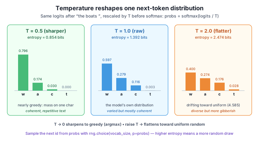
probs = softmax(logits / T). Lowering T to 0.5 concentrates mass on w (entropy 0.854 bits, near-greedy); T=1.0 is the model's raw distribution (1.392 bits); raising T to 2.0 flattens the bars toward one another (2.474 bits) on the way to the uniform ceiling of log2(24)=4.585 bits. The next id is then drawn with rng.choice(vocab_size, p=probs), so higher entropy means a more random draw.The generator is greedy’s loop with the choice function swapped out. We slice the last block_size ids as context, run one forward pass, divide the final-position logits by temperature, softmax them into probabilities, and draw the next id from that distribution with rng.choice. The rng is passed in so the caller controls the randomness (and reproducibility).
def generate(model, prompt, n_new, temperature, rng):
    block_size = model.cfg[1]                     # (vocab_size, block_size, n_embd, n_head, n_layer)
    ids = encode(prompt)
    for _ in range(n_new):
        context = np.array([ids[-block_size:]])   # (1, T), T <= block_size
        logits = model.forward(context)[0][0, -1] # (vocab_size,) next-char scores
        probs = softmax(logits / temperature)     # temperature-scaled distribution
        next_id = int(rng.choice(vocab_size, p=probs))   # weighted random draw
        ids.append(next_id)
    return decode(ids)
The only substantive line beyond greedy is probs = softmax(logits / temperature) followed by rng.choice(vocab_size, p=probs) instead of argmax. Everything else, the context slicing, the single forward pass, the append, is identical. Now generate from one prompt at three temperatures, seeding the rng the same way each time so the differences come from temperature alone, not from a different random stream.
for T in [0.5, 1.0, 1.5]:
    r = np.random.default_rng(42)                 # same seed each time
    print(f"T={T}:", repr(generate(model, "the boats ", 90, T, r)))
T=0.5: 'the boats wait outside the bay when the fog is thick. a small waifog the keeper counts the boats and'
T=1.0: 'the boats wait outside the bay when the fog is thome when the lantern glows. the boats wait outside '
T=1.5: 'the boats wait outside the bay when the fog is thome lantern anthe golows. the boats wait outside th'The three outputs are genuinely different in character, and the difference tracks the temperature exactly. At T=0.5 the text is almost entirely clean Lantern Bay prose, with only one small stumble ("a small waifog") where a low-probability draw slipped through. At T=1.0 the model samples from its raw distribution and takes a different branch after “the fog is th” ("thome" instead of “thick”), then recovers into coherent sentences, more varied than the low-temperature run but still readable. At T=1.5 the errors multiply: "thome lantern anthe golows" is starting to fray into non-words even though the overall rhythm of the corpus survives. Push it further and it comes apart completely.
print("T=2.0:", repr(generate(model, "the boats ", 90, 2.0, np.random.default_rng(42))))T=2.0: 'the boats wait outhe ske the lantern boars at mp keeper rings the bell when a boats at landrnf ar ni'At T=2.0 the flattened distribution keeps handing real probability to characters the model would normally reject, and the output degrades into misspellings and fragments: "outhe ske", "boars", "landrnf". This is the honest cost of high temperature. Flattening the distribution buys you diversity and surprise, but it also lets through characters the model has good reason to consider unlikely, and on a character-level model that shows up directly as broken spelling. There is no free lunch: coherence and variety pull against each other, and temperature is the dial that sets where you sit between them.
The whole motivation was to escape greedy’s one-completion-per-prompt determinism. Let us confirm we actually did. We draw twice from the same prompt at T=1.0, letting the rng advance between the two calls (so each draw uses fresh random numbers), and compare.
r = np.random.default_rng(7)
s1 = generate(model, "the lamp keeper ", 90, 1.0, r)
s2 = generate(model, "the lamp keeper ", 90, 1.0, r)   # same rng, advanced state
print("sample 1:", repr(s1))
print("sample 2:", repr(s2))
print("identical:", s1 == s2)
sample 1: 'the lamp keeper lights the lantern when then the fog is thick. a small boat drifts nime the when the fog r'
sample 2: 'the lamp keeper lights the lantern whenmmpe the lantern whenn then the fog rolls in. the boats come home w'identical: Falseidentical: False. Two runs, one prompt, two different continuations, exactly what greedy could never do. The two samples share their opening (both start “the lamp keeper lights the lantern when”) because near the prompt the distribution is sharply peaked and both draws take the same high-probability path, but they diverge the moment they hit a position where the model is less certain and the dice land differently. That branch-point divergence is stochastic generation working as intended.
This does not mean the output is unreproducible. Randomness in NumPy comes from the rng, so a fixed seed gives a fixed stream and therefore a fixed result. Reseed identically and you get byte-identical text every time.
a = generate(model, "the tide ", 60, 1.5, np.random.default_rng(123))
b = generate(model, "the tide ", 60, 1.5, np.random.default_rng(123))
print("same-seed identical:", a == b)
same-seed identical: TrueSo sampling gives you variety when you want it (advance or change the seed) and exact reproducibility when you need it (reuse the seed). That combination, controllable randomness, is why every real text generator is built on seeded sampling rather than either pure determinism or uncontrolled noise.
Temperature is a generation-time knob, not a training change
Nothing above retrained the model. The weights are frozen; temperature only rescales the logits at sampling time, so you can pick a different T for every request without touching the network. That is why production systems expose temperature as a per-call parameter: the same trained model can be run conservative (T around 0.7) for factual answers and loose (T above 1.0) for brainstorming, just by changing the divisor in softmax(logits / T).
Exercise 1. Verify the temperature-zero limit numerically. You cannot divide by exactly zero, but you can approach it: compute softmax(logits / T) for the "the boats " logits at T = 0.1, T = 0.01, and T = 0.001, and print the maximum probability and the argmax index each time. Confirm the maximum probability climbs toward 1.0 and its index matches logits.argmax(). Explain in one sentence why this proves low-temperature sampling collapses into greedy decoding.
Hint
Reuse logits = model.forward(context)[0][0, -1]. For each tiny T, compute p = softmax(logits / T) and print p.max() and p.argmax(). As T shrinks the gap between the top logit and the rest is multiplied up without bound, so p.max() approaches 1.0 and every other probability approaches 0. Since rng.choice can only return an index with nonzero probability, it is forced to return logits.argmax(), which is exactly greedy’s choice.
Exercise 2. Plot entropy against temperature as a table. Loop over T in [0.25, 0.5, 0.75, 1.0, 1.5, 2.0, 4.0], compute entropy_bits(softmax(logits / T)) for the same fixed logits, and print each (T, entropy) pair. Confirm entropy increases monotonically with T and compare the largest value against the uniform ceiling log2(24). Why does entropy never quite reach that ceiling for any finite T?
Hint
Entropy rises with T because flattening the distribution spreads probability toward the uniform one, which has the maximum entropy of any distribution over 24 outcomes. It only equals log2(24) in the T \to \infty limit, where every scaled logit becomes indistinguishable from zero; for any finite T the original logit gaps are shrunk but never fully erased, so a little structure always remains and entropy stays just below the ceiling.
Exercise 3. Quantify the coherence cost of temperature. Write a helper in_corpus_rate(text) that returns the fraction of length-4 substrings of text that appear somewhere in CORPUS (a rough “how much of this looks like real Lantern Bay text” score). Generate 200 characters from "the " at T = 0.5, 1.0, and 2.0 (fixed seed) and print the rate for each. Confirm the rate falls as temperature rises, and connect that number to the misspellings you saw in the printed samples.
Hint
For the helper, slide a window: sum(1 for i in range(len(text)-3) if text[i:i+4] in CORPUS) / (len(text)-3). A 4-gram that appears in CORPUS is a short stretch of genuinely learned text; a 4-gram that does not is usually a misspelling or a bad join. As T climbs, the flattened distribution admits more improbable characters, so more 4-grams fall outside the corpus and the rate drops, the numeric version of “high temperature produces more gibberish.”
Temperature sampling replaces greedy’s argmax with a weighted random draw from the model’s next-token distribution, and adds one knob to control how spread out that distribution is. You sample with rng.choice(vocab_size, p=probs) where probs = softmax(logits / T), so dividing the logits by T before the softmax sharpens the distribution when T < 1 (mass concentrates, near-greedy) and flattens it when T > 1 (mass spreads, near-uniform). You measured the effect as entropy on a real distribution, 0.854 bits at T=0.5 rising to 2.474 bits at T=2.0, and read it in real output: T=0.5 gave clean Lantern Bay prose, T=1.5 began to misspell, and T=2.0 degraded into fragments. Two draws at T=1.0 produced different completions, proving generation is now stochastic, while a fixed seed kept it reproducible.
rng.choice(vocab_size, p=probs) instead of taking argmax; this is what makes generation stochastic.T applied as softmax(logits / T); it rescales the logit gaps without changing their ranking.T < 1 concentrates mass on the top tokens (toward greedy), T = 1 is the raw distribution, T > 1 spreads mass out (toward uniform).T \to 0 recovers greedy argmax; T \to \infty recovers the uniform distribution.0.854 to 2.474 bits as T rose from 0.5 to 2.0, bounded by the uniform ceiling log2(24) = 4.585.T is coherent but repetitive, high T is varied but produces more misspellings; there is no setting that maximizes both.Temperature is the single most-used generation control in practice: every deployed language model exposes it, and choosing it well is the difference between a chatbot that sounds robotic and one that sounds unhinged. Because it acts only on the logits at sampling time, one frozen model can be conservative for factual work and loose for creative work just by changing a divisor, no retraining required. Building it from scratch also makes the abstraction concrete: you can see that “creativity” in a language model is not a mysterious property but a measurable amount of entropy in a distribution you can dial up or down. And watching high temperature slide into misspellings on your own tiny model is the clearest possible illustration of why raw temperature alone is a blunt instrument, it flattens everything, including characters that should stay near zero, which is exactly the weakness the next tools are designed to fix.
You now have a real knob for the coherence-versus-variety trade-off, but you also saw its flaw: pushing temperature up to get variety also hands probability to characters the model has good reason to reject, and the text frays into misspellings. The problem is that temperature reshapes the whole distribution at once, it cannot say “give me variety among the plausible options but never touch the junk in the long tail.” The next lesson introduces top-k sampling, which attacks exactly that. Before sampling, you will keep only the k highest-probability characters, set the rest to zero, and renormalize, so the model can still be adventurous among its top few candidates while the implausible tail is cut off entirely. You will implement the top-k filter in NumPy, watch it hold coherence at temperatures that made plain sampling break down, and see how k and temperature combine into a sharper pair of controls than either one alone.
Keep DATATWEETS free. Help fund practical data, AI, and engineering lessons for learners worldwide.
