Lesson 4 - Top-p (Nucleus) Sampling

Welcome to Top-p (Nucleus) Sampling#

In the last lesson you built top-k sampling: at each step you kept the k most likely next characters, zeroed out the rest, renormalized, and sampled. That was a real improvement over plain temperature sampling because it hard-blocks the long tail of junk tokens that should never be chosen. But top-k has a quiet weakness, and it comes from the one thing that makes it simple: k is a fixed number.

A fixed k cannot know the shape of the distribution it is filtering. Sometimes your MiniGPT is almost certain what comes next, and k lets in nine characters that all deserve a probability of essentially zero. Other times the model is honestly torn between several good continuations, and k chops off options it should have kept. This lesson introduces top-p sampling, also called nucleus sampling, which chooses how many tokens to keep per step based on the probabilities themselves. You will implement it in pure NumPy on the same trained model and watch the kept-count change with the distribution.

By the end of this lesson, you will be able to:

• Explain why a fixed k is simultaneously too loose on peaked distributions and too tight on flat ones
• Define the nucleus: the smallest set of top tokens whose cumulative probability reaches a threshold p
• Implement top_p_filter(logits, p) in NumPy by sorting, taking a cumulative sum, and cutting at the crossing point
• Measure on two real next-token distributions from your model how many tokens the nucleus keeps at p = 0.9
• Generate text with nucleus sampling and compare a top-p sample against a top-k sample

You should have the trained MiniGPT from Module 7 and the top-k filter from the previous lesson fresh in mind, along with softmax, encode, and decode. Let’s fix the fixed-k problem.

The problem with a fixed k#

Recall what a next-token distribution can look like. After a forward pass we take the final-position logits, logits[0, -1], and apply softmax to get a probability for each of the 24 characters in our vocabulary. On our Lantern Bay corpus the shape of that distribution swings wildly from one context to the next.

Consider two extremes:

• A peaked context. After "...the tide is low. t", the only character that ever follows in the corpus is h (as in the). The model has learned this cold: it puts essentially all of its probability on h. Every other character is noise. Here k = 10 would keep nine characters the model has already ruled out. Sampling among them can only hurt.
• A flat context. After "...rises at dusk and fa", the corpus genuinely continues several ways (falls, and the model also entertains other plausible letters). Probability is spread across four or five characters that each deserve a real shot. Here a small k, say k = 2, would throw away good options and make the text more repetitive than it needs to be.

No single k is right for both. The distribution’s shape is the information top-k ignores. What we actually want is a rule phrased in the currency the model speaks: probability mass. Keep enough of the most likely tokens to cover, say, 90% of the probability, and drop the rest, however many that turns out to be.

The nucleus: cumulative probability up to p#

Here is the rule precisely. Fix a threshold p, for example p = 0.9. To build the nucleus:

1. Sort the token probabilities in descending order.
2. Walk down the sorted list, keeping a running cumulative sum.
3. Keep tokens until the cumulative sum first reaches (crosses or equals) p, including the token that crosses it.
4. Drop every token after that. Renormalize the kept probabilities so they sum to 1, then sample.

The mathematics is just a running total. If $q_1 \ge q_2 \ge \dots \ge q_V$ are the sorted probabilities, the nucleus is the smallest prefix of size $n$ such that

Because we always include the token that tips the sum past p, the kept mass is at least p, never less. And because the list is sorted, the nucleus is always the smallest such set: no cheaper way to cover p exists.

Notice what this buys us. On a peaked distribution the very first token might already hold 0.99 of the mass, so n = 1 and we are done. On a flat distribution no single token clears p, so n grows until enough small contributions add up. The count $n$ is an output of the distribution, not a hyperparameter you guessed. That single change is the whole idea of nucleus sampling.

Setting up the trained model#

Everything below runs on the MiniGPT you built and trained in earlier modules, on the canonical Lantern Bay corpus. We train a small model briefly so the demo is fully reproducible, then reuse it for every experiment in this lesson.

import numpy as np, warnings
warnings.filterwarnings("ignore")

CORPUS = (
    "the lamp keeper walks the shore at dusk. "
    "the lamp keeper lights the lantern when the fog rolls in. "
    "the boats come home when the lantern glows. "
    "the boats wait outside the bay when the fog is thick. "
    "a small boat drifts near the rocks at dawn. "
    "the keeper rings the bell when a boat drifts near the rocks. "
    "the tide rises at dusk and falls at dawn. "
    "the gulls call over the bay when the tide is low. "
    "the keeper counts the boats and writes the count in a book. "
    "the lantern burns all night and rests at dawn. "
) * 20
chars = sorted(set(CORPUS)); vocab_size = len(chars)
stoi = {c: i for i, c in enumerate(chars)}
itos = {i: c for i, c in enumerate(chars)}
encode = lambda s: [stoi[c] for c in s]
decode = lambda ids: "".join(itos[i] for i in ids)
data = np.array(encode(CORPUS), dtype=np.int64)

# MiniGPT, Adam, get_batch, softmax: unchanged from Modules 2-7 (imported here).
model, final_loss = train()          # 1000 Adam steps, lr = 3e-3, seed 42
print("vocab_size", vocab_size, "| final train loss", round(final_loss, 4))

vocab_size 24 | final train loss 0.1621

The model reaches a train loss of about 0.16, low enough that its next-token distributions are sharp where the corpus is predictable and spread out where it is not, which is exactly the contrast we want to probe.

Implementing top_p_filter#

The filter mirrors the top-k filter you already wrote, but instead of slicing at a fixed index it slices where the cumulative sum crosses p. We return the filtered logits (with dropped tokens set to $-\infty$ so softmax sends them to zero) and the indices we kept, so we can inspect the nucleus size.

def softmax(x, axis=-1):
    x = x - x.max(axis=axis, keepdims=True)
    e = np.exp(x)
    return e / e.sum(axis=axis, keepdims=True)

def top_p_filter(logits, p):
    probs = softmax(logits)
    order = np.argsort(probs)[::-1]           # indices, most likely first
    sorted_probs = probs[order]
    cumulative = np.cumsum(sorted_probs)      # running total down the sorted list
    # keep up to AND INCLUDING the token that crosses p
    cutoff = np.searchsorted(cumulative, p) + 1
    cutoff = min(cutoff, len(probs))
    keep = order[:cutoff]
    filtered = np.full_like(logits, -np.inf)
    filtered[keep] = logits[keep]
    return filtered, keep

def next_probs(model, ids):
    ctx = np.array([ids[-model.cfg[1]:]])     # last block_size tokens
    logits, _ = model.forward(ctx)
    return logits[0, -1]                       # final-position logits

The one subtle line is np.searchsorted(cumulative, p) + 1. Since cumulative is sorted ascending, searchsorted returns the index where p would be inserted, that is, the count of entries strictly below p. Adding 1 includes the token that crosses the threshold, giving us the smallest prefix whose mass is at least p. Setting dropped logits to -np.inf rather than a large finite value guarantees they contribute exactly zero after softmax.

Watching the nucleus adapt#

Now the payoff. We scan many real contexts from the corpus, measure the entropy of the model’s next-token distribution at each, and pick the most peaked and the most uncertain. Then we ask top_p_filter how many tokens it keeps at p = 0.9 for each.

# scan contexts; find the most peaked (low entropy) and most uncertain (high entropy)
rng_scan = np.random.default_rng(0)
n_data = int(len(data) * 0.9)
best_peak = best_flat = None
for _ in range(300):
    i = int(rng_scan.integers(0, n_data - 40))
    ids = list(data[i:i+32])
    probs = softmax(next_probs(model, ids))
    ent = -np.sum(probs * np.log(probs + 1e-12))
    if best_peak is None or ent < best_peak[0]: best_peak = (ent, ids)
    if best_flat is None or ent > best_flat[0]: best_flat = (ent, ids)

for label, (ent, ids) in [("PEAKED", best_peak), ("UNCERTAIN", best_flat)]:
    probs = softmax(next_probs(model, ids))
    _, keep = top_p_filter(next_probs(model, ids), 0.9)
    top3 = np.argsort(probs)[::-1][:3]
    print(f"{label:9} entropy={ent:.3f}  nucleus(p=0.9) keeps {len(keep)} tokens")
    print("   context tail:", repr(decode(ids[-20:])))
    print("   top-3:", [(itos[int(t)], round(float(probs[t]), 3)) for t in top3])

PEAKED    entropy=0.000  nucleus(p=0.9) keeps 1 tokens
   context tail: 'n the tide is low. t'
   top-3: [('h', 1.0), ('i', 0.0), ('s', 0.0)]
UNCERTAIN entropy=1.553  nucleus(p=0.9) keeps 4 tokens
   context tail: 'rises at dusk and fa'
   top-3: [('l', 0.292), ('f', 0.282), ('w', 0.238)]

There it is, with real numbers from your own model. After "...the tide is low. t" the model is certain the next character is h: it holds essentially all the mass, so the nucleus is 1 token. A fixed k = 10 here would have carried nine dead characters. After "...rises at dusk and fa" the model spreads its bets, no single character clears 0.3, and the nucleus grows to 4 tokens. Same p = 0.9, same code, and the kept count moved from 1 to 4 on its own.

Reading the cumulative sum directly#

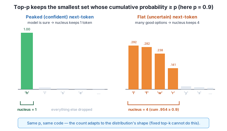
To make the crossing concrete, here is the running total on the uncertain distribution. The nucleus stops at the first row where the cumulative sum reaches 0.9.

_, ids = best_flat
probs = softmax(next_probs(model, ids))
order = np.argsort(probs)[::-1]
cum = np.cumsum(probs[order])
print("rank char  prob    cum")
for r in range(6):
    t = int(order[r])
    print(f"{r:>4}  {itos[t]!r}   {probs[order][r]:.3f}   {cum[r]:.3f}")

rank char  prob    cum
   0  'l'   0.292   0.292
   1  'f'   0.282   0.575
   2  'w'   0.238   0.813
   3  'r'   0.141   0.954
   4  'y'   0.019   0.973
   5  's'   0.014   0.987

The cumulative sum reaches 0.813 after three tokens, still short of 0.9, so r is pulled in and the total lands at 0.954. That fourth token is the one that crosses the threshold, so the nucleus is exactly those four; y and everything after are dropped. This is the entire algorithm, visible in one column of numbers.

Generating with nucleus sampling#

Wrapping the filter in the autoregressive loop is straightforward: at each step, filter the final-position logits, softmax to renormalize the survivors, and sample one token with np.random.default_rng. Seeding the generator keeps the whole run reproducible.

def generate_top_p(model, prompt_ids, n, p, rng):
    ids = list(prompt_ids)
    for _ in range(n):
        filtered, _ = top_p_filter(next_probs(model, ids), p)
        probs = softmax(filtered)
        ids.append(int(rng.choice(len(probs), p=probs)))
    return ids

seed_ids = encode("the ")
out_p = generate_top_p(model, seed_ids, 80, 0.9, np.random.default_rng(42))
print("TOP-P p=0.9:", repr(decode(out_p)))

again = generate_top_p(model, seed_ids, 80, 0.9, np.random.default_rng(42))
print("reproducible:", decode(out_p) == decode(again))

TOP-P p=0.9: 'the rocks. the tide rises at dusk and faftsk and fafalls at dawn. the gulls cal over'
reproducible: True

The output stays firmly in the Lantern Bay vocabulary, wanders across several sentences instead of parroting one, and reproduces byte-for-byte on a re-run with the same seed. On the peaked stretches ("the tide rises at dusk and fa...") the nucleus was collapsing to a single token, so the model followed the corpus faithfully; on the uncertain stretches it had room to vary, which is where the small slips like faft and cal come from, a tiny 2-layer model on 24 characters, doing its honest best.

Top-p versus top-k, side by side#

For contrast, here is a top-k sample with k = 5 from the identical model, prompt, and seed.

def generate_top_k(model, prompt_ids, n, k, rng):
    ids = list(prompt_ids)
    for _ in range(n):
        logits = next_probs(model, ids)
        keep = np.argsort(logits)[::-1][:k]
        filtered = np.full_like(logits, -np.inf)
        filtered[keep] = logits[keep]
        probs = softmax(filtered)
        ids.append(int(rng.choice(len(probs), p=probs)))
    return ids

out_k = generate_top_k(model, seed_ids, 80, 5, np.random.default_rng(42))
print("TOP-K k=5 :", repr(decode(out_k)))

TOP-K k=5 : 'the lantern burns all night and rests at dawn. the lamp keeper lights the lantern wh'

Both strategies produce clean text on this corpus, because the corpus is small and low-entropy. The difference is not always visible in a single sample; it is structural. Top-k always carries exactly five candidates, even when the model is certain (wasting four slots) and even when it is torn among six good options (dropping one). Top-p carried one token where the model was sure and four where it was not, spending its randomness only where the model actually had a choice. On a large, high-entropy corpus that adaptivity is what keeps generation both varied and on-topic, which is why nucleus sampling became the default decoding strategy for large language models.

Practice Exercises#

Exercise 1. Rewrite top_p_filter without np.searchsorted, using an explicit loop that accumulates probability and breaks once the running total reaches p. Confirm on the uncertain distribution (best_flat) that it returns the same four kept indices as the vectorized version.

Exercise 2. Measure how the nucleus size responds to p. For the uncertain distribution best_flat, print len(keep) for p in [0.5, 0.7, 0.9, 0.99]. Then do the same for the peaked distribution best_peak and explain why one of them barely moves.

Exercise 3. Add temperature to nucleus sampling. Modify generate_top_p to divide the logits by a temp argument before calling top_p_filter, and generate with temp=0.7 and temp=1.3 at p = 0.9. Describe how temperature and p interact on the kept count.

Summary#

You replaced the fixed cutoff of top-k with a threshold on probability mass. By sorting the next-token probabilities, taking a cumulative sum, and keeping the smallest prefix that reaches p, you built a filter whose kept-count adapts to each distribution: 1 token where your MiniGPT was certain, 4 tokens where it was uncertain, all at the same p = 0.9. You saw the crossing happen in a single column of cumulative numbers, generated reproducible text with nucleus sampling, and compared it against a top-k sample to see why the adaptivity matters.

Key Concepts#

• Top-p (nucleus) sampling keeps the smallest set of top tokens whose cumulative probability reaches p, then renormalizes and samples from them.
• The nucleus size is an output, not a hyperparameter. It shrinks on peaked distributions and grows on flat ones, unlike the fixed k of top-k sampling.
• Mechanics: sort probabilities descending, take np.cumsum, and cut at the first index where the running total reaches p, including the crossing token so the kept mass is at least p.
• Renormalize after filtering. Dropped logits set to $-\infty$ become zero under softmax; the survivors must be re-softmaxed so they sum to 1 before sampling.
• Top-p and top-k are complementary. Top-p adapts to shape; capping the nucleus with a k guards against an unusually flat tail. Temperature composes with both by reshaping the logits first.

Why This Matters#

A fixed k treats a confident model and a hesitant one identically, which is the wrong thing to do: it wastes probability on dead tokens when the model is sure and starves good options when it is torn. Nucleus sampling ties the amount of randomness to the model’s own confidence, spending exploration only where the model genuinely has a choice. That is why top-p, often combined with temperature and a k cap, is the decoding strategy behind most production language models. Having built it from a cumulative sum in NumPy, you now understand exactly what that one line in a generation config is doing.

Continue Building Your Skills#

You now have a full toolkit of decoding strategies, greedy, temperature, top-k, and top-p, each implemented in pure NumPy on the model you trained from scratch. In the next lesson you will pull them together into a single reusable text-generator project: one generate function that accepts a prompt, a temperature, and optional top-k and top-p settings, wraps your MiniGPT, and streams out characters one at a time. You will turn the scattered experiments of this module into a clean, configurable interface you can point at any prompt and any combination of sampling controls, the piece that finally makes your from-scratch transformer feel like something you can actually write with.