Lesson 1 - Why One Head Isn't Enough

Welcome to Why One Head Isn’t Enough#

In Module 2 you built a single self-attention head from scratch: you projected the input into queries, keys, and values, scored every query against every key, softmaxed the scores into weights, and mixed the values. That one head is the engine of the tiny GPT you are assembling. But there is a quiet limitation hiding inside it, and this module exists to fix it.

A single head has exactly one set of projection matrices, Wq, Wk, and Wv. Those three matrices decide, once and for all, what counts as “relevant.” So for any query position, the head produces a single attention distribution, one row of weights that sums to 1. It has one opinion about where to look. If a language needs to track both the word right before the current one and a matching word far back in the sentence, a lone head cannot do both at once. It has to pick.

By the end of this lesson, you will be able to:

• Explain why a single attention head can express only one attention pattern per position
• Describe how multiple heads, each with their own Wq, Wk, Wv, add representational capacity cheaply
• Build two independent attention heads in NumPy over the same input sequence
• Show quantitatively that two heads attend differently: compare their attention matrices, the max absolute weight gap, and their per-row argmax
• Motivate the mechanics you will implement next: splitting, parallel attention, and combining head outputs

You should be comfortable with the single-head forward pass from Module 2 and with NumPy matrix multiplication. Let’s see exactly where one head runs out of room.

One Head, One Opinion#

Recall the shape of a single head. Activations flow as $(B, T, C)$: batch $B$, sequence length $T$, model width $C$. The head projects the input $X$ into three $(B, T, hs)$ tensors, scores them, and returns weighted values:

The weights matrix is $(B, T, T)$: for each of the $T$ query positions, one row of $T$ numbers that sum to 1, describing how much that position draws from every other position. That row is the head’s opinion. And because it is produced entirely by Wq, Wk, and Wv, there is only one of it. Train the head to attend to the previous token and it gets good at that and only that. Train it to hunt for repeated words and it forgets about neighbors. One head, one specialization.

Here is an analogy. Imagine handing the same sentence to several people and asking each to underline something different: one underlines the word before each noun, another underlines every place a word repeats, a third underlines punctuation. Each reader produces a different set of underlines. If you only had one reader, you would get one kind of underline and miss the rest. Multi-head attention is hiring several readers and pooling their notes.

Each head is cheap because we make the heads narrow: instead of one head of width $C$, we run $h$ heads each of width $hs = C / h$. The total amount of projection work stays about the same, but now there are $h$ independent sets of Wq, Wk, Wv, so the model can express $h$ different attention patterns per position at once. That is the whole trade: same budget, many more views. This lesson proves the “different views” claim with real numbers; the rest of the module builds the splitting and combining machinery.

Setting Up Two Heads Over One Sentence#

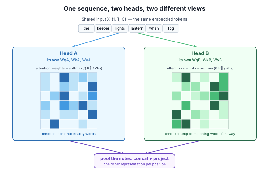
To make the argument concrete, we take a short slice of the Lantern Bay corpus, embed it once, and feed that single embedded sequence into two independent heads. Each head gets its own Wq, Wk, Wv, drawn from the same seeded random stream but never shared. If two heads attend differently even with no training at all, then the capacity for different views is built in from the start; training only sharpens it.

We tokenize the slice one token per word so the attention matrix is small enough to read cell by cell. We seed everything with np.random.seed(42) and use a demo init of * 0.3 on the projections, with unit-scale word embeddings. As the shared brief notes, real transformers initialize projections near * 0.02, but at that scale the softmax comes out almost uniform and there is nothing to inspect. A slightly larger init lets the two heads differentiate visibly, which is exactly what we want to see here.

import numpy as np

def softmax(x, axis=-1):
    x = x - x.max(axis=axis, keepdims=True)
    e = np.exp(x)
    return e / e.sum(axis=axis, keepdims=True)

def attention(X, Wq, Wk, Wv):
    Q, K, V = X @ Wq, X @ Wk, X @ Wv                  # each (B, T, hs)
    hs = Q.shape[-1]
    scores = Q @ K.transpose(0, 2, 1) / np.sqrt(hs)   # (B, T, T)
    weights = softmax(scores, axis=-1)                # (B, T, T)
    return weights @ V, weights                       # out: (B, T, hs)

# a short Lantern Bay slice, one token per word
sentence = "the keeper lights the lantern when fog rolls"
words = sentence.split()
vocab = sorted(set(words))
stoi = {w: i for i, w in enumerate(vocab)}
ids = np.array([[stoi[w] for w in words]])            # (1, T)
T = len(words)
print("words:", words)
print("T:", T)

words: ['the', 'keeper', 'lights', 'the', 'lantern', 'when', 'fog', 'rolls']
T: 8

The slice has eight word-tokens (the word the appears twice, which is deliberate, it gives the heads a repeated token to potentially latch onto). Now embed the tokens once and build the two heads. The forward variables stay named Q, K, V; only the weight matrices carry a head suffix.

np.random.seed(42)
C = 16     # model width
hs = 8     # head size for this demo

# fixed word-embedding table, unit scale so tokens are distinct
Emb = np.random.randn(len(vocab), C) * 1.0
X = Emb[ids]                                          # (1, T, C)
print("X shape:", X.shape)

# Head A: its own projections (demo init * 0.3 so patterns differentiate)
WqA = np.random.randn(C, hs) * 0.3
WkA = np.random.randn(C, hs) * 0.3
WvA = np.random.randn(C, hs) * 0.3

# Head B: a completely separate set of projections
WqB = np.random.randn(C, hs) * 0.3
WkB = np.random.randn(C, hs) * 0.3
WvB = np.random.randn(C, hs) * 0.3

outA, wA = attention(X, WqA, WkA, WvA)
outB, wB = attention(X, WqB, WkB, WvB)
print("outA shape:", outA.shape, "| wA shape:", wA.shape)

X shape: (1, 8, 16)
outA shape: (1, 8, 8) | wA shape: (1, 8, 8)

Both heads consume the identical X. Each produces an $(1, 8, 8)$ attention matrix, one row per query word, one column per key word. The only difference between them is the six random projection matrices. If those alone are enough to pull the two attention patterns apart, the case for multiple heads is made.

Proving the Two Heads Attend Differently#

Print both attention matrices and measure how far apart they are. We round to two decimals for readability and report the largest single-cell disagreement.

np.set_printoptions(precision=2, suppress=True)
print("Head A attention matrix (rows = query word, cols = key word):")
print(wA[0])
print("Head B attention matrix:")
print(wB[0])

max_diff = np.abs(wA[0] - wB[0]).max()
print("max abs difference between the two heads:", round(float(max_diff), 4))

Head A attention matrix (rows = query word, cols = key word):
[[0.12 0.07 0.28 0.12 0.1  0.14 0.09 0.09]
 [0.09 0.01 0.19 0.09 0.05 0.04 0.34 0.2 ]
 [0.04 0.18 0.33 0.04 0.09 0.29 0.03 0.02]
 [0.12 0.07 0.28 0.12 0.1  0.14 0.09 0.09]
 [0.13 0.   0.29 0.13 0.22 0.14 0.07 0.01]
 [0.11 0.01 0.1  0.11 0.09 0.07 0.44 0.07]
 [0.1  0.14 0.19 0.1  0.15 0.18 0.04 0.1 ]
 [0.02 0.78 0.04 0.02 0.04 0.06 0.   0.04]]
Head B attention matrix:
[[0.07 0.22 0.1  0.07 0.05 0.31 0.1  0.09]
 [0.05 0.13 0.13 0.05 0.03 0.06 0.26 0.29]
 [0.11 0.08 0.1  0.11 0.09 0.17 0.15 0.18]
 [0.07 0.22 0.1  0.07 0.05 0.31 0.1  0.09]
 [0.08 0.01 0.25 0.08 0.04 0.11 0.34 0.09]
 [0.11 0.   0.31 0.11 0.03 0.23 0.18 0.03]
 [0.15 0.28 0.04 0.15 0.17 0.14 0.03 0.03]
 [0.01 0.89 0.   0.01 0.06 0.01 0.   0.01]]
max abs difference between the two heads: 0.2617

These are two genuinely different matrices. The largest single-cell gap is 0.2617, more than a quarter of the entire probability budget for a row moved from one word to another. Look at the second row (the query word keeper): Head A puts its heaviest weight, 0.34, on column 6 (fog), while Head B splits its mass toward columns 6 and 7 (fog and rolls) with 0.26 and 0.29. Same query word, same input, two different reads.

The cleanest summary is where each head points: the column with the maximum weight in each row, translated back to the word it lands on.

amA = wA[0].argmax(axis=1)
amB = wB[0].argmax(axis=1)
print("Head A: each word's top focus ->", [words[j] for j in amA])
print("Head B: each word's top focus ->", [words[j] for j in amB])
print("rows where the two heads disagree:", int((amA != amB).sum()), "of", T)

Head A: each word's top focus -> ['lights', 'fog', 'lights', 'lights', 'lights', 'fog', 'lights', 'keeper']
Head B: each word's top focus -> ['when', 'rolls', 'rolls', 'when', 'fog', 'lights', 'keeper', 'keeper']
rows where the two heads disagree: 7 of 8

On 7 of the 8 query positions the two heads pick a different word as most relevant. Head A keeps drifting back toward lights; Head B fans out across when, rolls, keeper, and others. Neither pattern is “right” here, these heads are untrained, but that is the point: with nothing but different random projections, the two heads already produce two distinct views of the same sentence. Give a real training signal, and each head is free to sharpen its own view into a useful specialization. One head could never hold all of those views at once.

From Two Heads to h Heads#

Two heads gave two views. The generalization is immediate: $h$ heads give $h$ views, each with its own Wq, Wk, Wv, all reading the same input in parallel. The tiny-GPT config for this course uses n_head = 4 with n_embd = 64, so each head is $hs = 64 / 4 = 16$ wide, and the layer produces four independent attention patterns per position instead of one.

But two questions remain, and they are the subject of the next lessons. First, where do the $h$ narrow heads come from, do we really run four separate projections, or is there a slicker way to carve one wide projection into four? Second, once the heads have each produced their own $(B, T, hs)$ output, how do we fuse those back into a single $(B, T, C)$ representation the rest of the network can use? The figure hinted at the answer, “concatenate and project”, and that is exactly the pooling step we build next. For now, hold on to the demonstrated fact: multiple heads are multiple opinions, and a model that can hold several opinions at once is strictly more expressive than one that can hold only one.

Practice Exercises#

Try these before checking the hints. They reuse the attention, softmax, X, and word setup from above.

Exercise 1: Add a Third Head#

Create a third head with its own WqC, WkC, WvC (same * 0.3 init, drawn right after Head B so the seed stays fixed), run it on the same X, and print its per-row argmax focus words. Confirm at least one row where all three heads point at three different words.

# Your code here (reuse attention, X, C, hs, words)

Exercise 2: Shrink the Init and Watch the Heads Blur Together#

Rebuild both heads with the projections scaled by * 0.02 instead of * 0.3, keeping everything else the same. Recompute the max absolute difference between the two attention matrices and explain in a comment why it collapses toward zero.

# Your code here: same setup, but * 0.02 on every projection

Exercise 3: Confirm Every Row Is a Valid Distribution#

For both heads, verify that each row of the attention matrix sums to 1 (softmax guarantees this, but proving it builds the habit). Print the per-row sums for Head A and check them against a vector of ones.

# Your code here: check that wA[0] and wB[0] rows each sum to 1

Summary#

You saw precisely where a single attention head runs out of room, and you proved with real NumPy that independent heads fix it. Let’s review.

Key Concepts#

The Bottleneck

• A single head has one Wq, one Wk, one Wv, so it produces exactly one attention distribution per query position, one opinion about relevance
• It cannot simultaneously track a nearby word and a matching word far away; it must specialize in one pattern

The Fix: Multiple Heads

• Run $h$ narrow heads of size $hs = C / h$, each with its own Wq, Wk, Wv, in parallel over the same input
• $h$ heads give $h$ different attention patterns per position, more representational capacity for about the same projection budget
• The analogy: several readers each underline a different pattern in the same sentence, then you pool their notes

What the Demo Showed (seed 42, demo init * 0.3)

• Two independent heads over the same 8-word Lantern Bay slice produced two different $(1, 8, 8)$ attention matrices
• Max absolute weight difference between them: 0.2617
• The heads disagreed about the top-focus word on 7 of 8 query positions
• Fully reproducible: no training, no shared projections, just different random Wq/Wk/Wv

Why This Matters#

Multi-head attention is not a minor tweak; it is one of the reasons transformers work as well as they do. Real trained models develop heads that specialize in strikingly interpretable ways, some track the previous token, some connect subjects to their verbs, some copy rare words forward, some attend to punctuation or sentence boundaries. All of that lives in the same layer, running in parallel, because each head has its own projections and its own opinion. You just demonstrated the seed of that behavior from scratch: change nothing but the projection matrices and the attention pattern changes with it. When you later inspect a trained model and see one head doing something a single-head model never could, you will know exactly why the capacity was there.

Continue Building Your Skills#

You have the motivation nailed down: many heads beat one because each head is an independent view, and you measured that independence directly. The natural next question is mechanical, how do we actually create $h$ heads without paying for $h$ full-width projections? In the next lesson you will learn head splitting: instead of building four separate $C \times hs$ matrices, you compute one wide $C \times C$ projection and then reshape the result into $h$ heads of size $hs$ along a new axis. It is a single reshape and transpose that turns one tensor into a stack of parallel heads, the efficient trick that lets a transformer run all its heads in one batched matmul. Master that reshape and you are most of the way to a working multi-head attention layer.