Lesson 2 - Splitting into Heads

Welcome to Splitting into Heads#

In the previous lesson you saw why a transformer wants several attention heads: each head can specialize, learning a different relationship between tokens. The obvious way to build that would be to keep h separate little projection matrices, run h separate attention calculations, and stack the results. It works, but it is clumsy, and it is not how real transformers (including the tiny char-level GPT you are building in this course) actually do it.

Instead they use one wide projection of shape (C, C) and then split the result into h heads with a reshape and a transpose. No extra matmuls, no Python loop over heads, just index arithmetic on a single tensor. This lesson is purely about that plumbing: how a (B, T, C) projection becomes a (B, h, T, hs) stack of independent per-head problems, and why the reshape and the transpose are each doing exactly what they need to.

By the end of this lesson, you will be able to:

• Explain why real transformers use one (C, C) projection instead of h small (C, hs) ones
• Compute the head size hs = C // h and say why C must divide evenly by h
• Reshape a (B, T, C) tensor into (B, T, h, hs) and read what each axis means
• Transpose to (B, h, T, hs) and explain why the head axis has to move
• Prove in NumPy that the split matches h separate projections and that it is fully invertible

You should already be comfortable with single-head self-attention from Module 2 and with NumPy array shapes. We will not score any attention here; that is Lesson 3. This lesson is the reshape mechanics that make it possible. Let’s begin.

One Wide Projection, Not h Small Ones#

Recall single-head self-attention. To build the query vectors you multiply the input X of shape (B, T, C) by a query weight Wq, and you get Q. For one head whose size is hs, that weight is (C, hs) and Q is (B, T, hs).

Multi-head attention wants h of these, each with its own hs-dimensional query, key, and value. The naive approach keeps h separate weights Wq0, Wq1, ..., Wq(h-1), each (C, hs), and runs the head loop by hand. Nothing is wrong with the math, but a matrix multiply is happiest as one big operation, and stacking h little (C, hs) matrices side by side gives you exactly one big (C, h * hs) matrix. Since we choose hs = C // h, that is just (C, C).

So the real design is: keep a single wide Wq of shape (C, C), do one matmul, and interpret the C output columns as h consecutive blocks of hs columns each. Block 0 is head 0’s query, block 1 is head 1’s query, and so on. The first hs columns of the wide Wq are literally head 0’s (C, hs) projection; the next hs columns are head 1’s. One matmul, h heads, and later in this lesson you will confirm that equivalence numerically.

The head size is fixed by the config:

with the constraint that C must be divisible by h. If it were not, the C columns could not be cut into h equal blocks and the reshape would fail outright. In our tiny-GPT config C = 64 and h = 4, so hs = 16, and 4 * 16 = 64 accounts for every column exactly.

The Reshape: (B, T, C) to (B, T, h, hs)#

After the wide projection, Q = X @ Wq has shape (B, T, C): for every example in the batch and every position in the sequence, a C-dimensional row. We want to reinterpret that C-dimensional row as h separate hs-dimensional head-rows lined up end to end.

That reinterpretation is exactly what reshape does. Because a reshape never moves data, only relabels how the flat buffer is indexed, splitting the last axis C into two axes (h, hs) is free:

Q_heads = Q.reshape(B, T, h, hs)   # (B, T, C) -> (B, T, h, hs)

Read the new shape (B, T, h, hs) axis by axis:

• B — which example in the batch.
• T — which position in the sequence.
• h — which head. This is the new axis carved out of C.
• hs — the coordinate inside that head’s vector.

The reason this split lands the columns in the right heads is the row-major memory order NumPy uses. The last axis varies fastest, so the flat C-length row is chopped into h contiguous chunks of length hs: columns 0..hs-1 become head 0, columns hs..2*hs-1 become head 1, and so on. That is precisely the block structure of the wide Wq from the previous section, which is why the two views agree.

The Transpose: (B, T, h, hs) to (B, h, T, hs)#

The reshape got the head axis to exist, but it is in an awkward place. In (B, T, h, hs) the head axis sits between the sequence axis T and the feature axis hs. If you want to treat each head as its own self-attention problem, you need each head to own a clean (T, hs) matrix, all T positions of that one head together. As laid out, head 0’s rows for different T positions are separated by the other heads’ data.

So we move the head axis up next to the batch axis with a transpose:

Q_split = Q_heads.transpose(0, 2, 1, 3)   # (B, T, h, hs) -> (B, h, T, hs)

The argument (0, 2, 1, 3) is the new order of the old axes: keep axis 0 (B) first, bring old axis 2 (h) into second place, send old axis 1 (T) to third, and keep axis 3 (hs) last. The result is (B, h, T, hs).

Now the last two axes are (T, hs): for a fixed batch index b and head index i, Q_split[b, i] is a complete (T, hs) matrix, one row per position, all belonging to head i. That is exactly the shape a single attention head expects. In Lesson 3 you will hand (B, h, T, hs) query, key, and value tensors straight to the scaled-dot-product machinery, and the B and h axes will just come along for the ride as batch dimensions. Grouping the head axis next to the batch axis is what makes that possible.

Doing It for Real in NumPy#

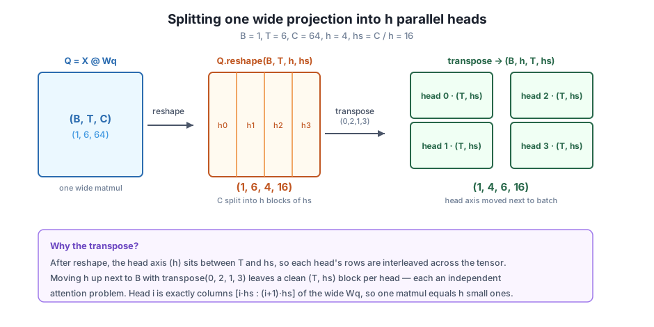
Time to make every shape concrete and prove the two claims that matter: that the split really does equal h separate (C, hs) projections, and that the whole reshape-plus-transpose is invertible so no information is lost or scrambled. We use a small input, B = 1, T = 6, C = 64, with h = 4 and hs = 16, and seed everything at 42.

import numpy as np

np.random.seed(42)

B, T, C = 1, 6, 64
h = 4
hs = C // h
print("B, T, C =", B, T, C)
print("h =", h, "| hs = C // h =", hs)
assert C % h == 0, "C must be divisible by h"

X = np.random.randn(B, T, C) * 0.1
Wq = np.random.randn(C, C) * 0.1
print("X shape: ", X.shape)
print("Wq shape:", Wq.shape)

B, T, C = 1 6 64
h = 4 | hs = C // h = 16
X shape:  (1, 6, 64)
Wq shape: (64, 64)

Wq is the single wide (64, 64) projection. We scale the init by 0.1 (rather than the training-scale 0.02) purely so the numbers are large enough to read; this lesson only inspects shapes and equality, so the scale is cosmetic. Now do the one matmul and the two steps:

Q = X @ Wq                          # (B, T, C)
print("Q = X @ Wq shape:          ", Q.shape)

Q_heads = Q.reshape(B, T, h, hs)    # split last axis into (h, hs)
print("reshape -> (B, T, h, hs):  ", Q_heads.shape)

Q_split = Q_heads.transpose(0, 2, 1, 3)   # move head axis up
print("transpose -> (B, h, T, hs):", Q_split.shape)

Q = X @ Wq shape:           (1, 6, 64)
reshape -> (B, T, h, hs):   (1, 6, 4, 16)
transpose -> (B, h, T, hs): (1, 4, 6, 16)

There is the full journey: (1, 6, 64) to (1, 6, 4, 16) to (1, 4, 6, 16). Every number is accounted for, since 6 * 64 = 384 = 4 * 6 * 16.

Now the first proof. Head i should equal projecting X by just columns i*hs : (i+1)*hs of the wide Wq. Let’s check all four heads:

match_all = True
for i in range(h):
    Wq_i = Wq[:, i*hs:(i+1)*hs]        # (C, hs): head i's slice of the wide matrix
    head_i_direct = X @ Wq_i           # (B, T, hs), computed separately
    head_i_split = Q_split[:, i, :, :] # (B, T, hs), pulled out of the split
    ok = np.allclose(head_i_direct, head_i_split)
    match_all = match_all and ok
    print(f"head {i}: split matches separate (C, hs) projection? {ok}")
print("all heads match:", match_all)

head 0: split matches separate (C, hs) projection? True
head 1: split matches separate (C, hs) projection? True
head 2: split matches separate (C, hs) projection? True
head 3: split matches separate (C, hs) projection? True
all heads match: True

Every head produced by the one-matmul-plus-split is bit-for-bit what you would get from an independent (C, hs) projection. That is the whole justification for the design: it is not an approximation, it is the same computation laid out more efficiently.

The second proof is invertibility. Undo the transpose (the same (0, 2, 1, 3) permutation is its own inverse here) and the reshape, and you should recover the original Q exactly:

Q_back = Q_split.transpose(0, 2, 1, 3).reshape(B, T, C)
print("recovered Q equals original Q exactly?", np.array_equal(Q_back, Q))
print("max abs diff:", np.abs(Q_back - Q).max())

recovered Q equals original Q exactly? True
max abs diff: 0.0

A difference of exactly 0.0 confirms the split moves no data and loses nothing; it is a pure reindexing. Re-running the entire script a second time prints identical shapes and identical True results, because the seed makes it fully deterministic.

Keys and Values Follow the Same Path#

Everything above was written for the query projection, but keys and values are identical in structure. Each has its own wide weight, Wk and Wv, both (C, C), and each goes through the same reshape-then-transpose to become (B, h, T, hs):

def split_heads(x, h):
    B, T, C = x.shape
    hs = C // h
    return x.reshape(B, T, h, hs).transpose(0, 2, 1, 3)   # (B, h, T, hs)

np.random.seed(42)
X = np.random.randn(1, 6, 64) * 0.1
Wq = np.random.randn(64, 64) * 0.1
Wk = np.random.randn(64, 64) * 0.1
Wv = np.random.randn(64, 64) * 0.1

Qh = split_heads(X @ Wq, 4)
Kh = split_heads(X @ Wk, 4)
Vh = split_heads(X @ Wv, 4)
print("Qh:", Qh.shape, "| Kh:", Kh.shape, "| Vh:", Vh.shape)

Qh: (1, 4, 6, 16) | Kh: (1, 4, 6, 16) | Vh: (1, 4, 6, 16)

Three tensors, all (1, 4, 6, 16), ready for attention. That small split_heads helper is the exact reshape logic your mini-GPT’s multi-head attention layer will call three times per block. In Lesson 3 you will feed these (B, h, T, hs) tensors into scaled-dot-product attention and watch all four heads score in parallel, treating B and h together as one big batch of independent attention problems.

Practice Exercises#

Try these before checking the hints. They reuse the B = 1, T = 6, C = 64, h = 4, hs = 16 setup and np.random.seed(42).

Exercise 1: Merge the Heads Back#

You have Q_split of shape (B, h, T, hs). Write the inverse of split_heads: a merge_heads(x, ) that returns to (B, T, C), and confirm with np.array_equal that merging Q_split recovers the original Q.

# Your code here: transpose the head axis back down, then reshape to (B, T, C)

Exercise 2: A Different Head Count#

Keep C = 64 but set h = 8. Compute the new hs, rerun the projection, reshape, and transpose, and print every shape. Then try h = 5 and observe what goes wrong.

# Your code here: repeat the split with h = 8, then attempt h = 5

Exercise 3: Prove Head 2 by Column Slice#

Without using Q_split, reconstruct head 2 directly: slice columns 2*hs : 3*hs out of the wide Wq, project X by that (C, hs) slice, and confirm with np.allclose that it equals Q_split[:, 2, :, :].

# Your code here: build Wq's head-2 column slice and compare to the split

Summary#

You learned the reshape plumbing that turns one wide projection into h parallel attention heads, the move that makes multi-head attention a single clean matmul instead of a Python loop. Let’s review.

Key Concepts#

One Wide Projection

• Real transformers use a single (C, C) weight for Wq (and Wk, Wv), not h separate (C, hs) weights
• The C output columns are h consecutive blocks of hs; block i is head i
• Head size is hs = C // h, and C must be divisible by h, or the reshape fails
• Merging the small projections into one changes nothing about the parameter count: h * C * hs = C * C

Reshape then Transpose

• reshape(B, T, h, hs) splits the last axis into a head axis and a within-head axis without moving data
• transpose(0, 2, 1, 3) lifts the head axis next to the batch axis, giving (B, h, T, hs)
• After the transpose, Q_split[b, i] is a clean (T, hs) matrix, one independent attention problem per head
• Reshape and transpose are not interchangeable: reshape regroups the flat buffer, transpose reorders axes

Proven in NumPy

• Each split head equals X @ Wq[:, i*hs:(i+1)*hs] exactly (all four heads matched)
• The full split is invertible: undo the transpose and reshape and recover Q with a max difference of 0.0
• With a fixed seed the shapes (1, 6, 64) -> (1, 6, 4, 16) -> (1, 4, 6, 16) are fully reproducible

Why This Matters#

Every real transformer, from the tiny char-level GPT in this course to the largest production models, splits into heads exactly this way. When you read a reference implementation and see .view(B, T, n_head, C // n_head).transpose(1, 2), that one line is the whole of this lesson: one wide projection, a reshape to carve out heads, a transpose to make each head an independent problem. Recognizing it means you can read multi-head attention code fluently and debug the shape errors that plague anyone who gets the reshape and transpose out of order.

It also sets up the payoff. Because the split leaves B and h as leading batch axes over clean (T, hs) matrices, the attention math you already wrote for a single head runs unchanged across all heads at once, with NumPy broadcasting over those leading axes. That is what the next lesson cashes in.

Continue Building Your Skills#

You now have h heads sitting side by side as a (B, h, T, hs) tensor, each a self-contained (T, hs) attention problem, and you proved the split is both faithful to h separate projections and perfectly reversible. In the next lesson, Lesson 3, you will run scaled-dot-product attention across all of those heads simultaneously: the Q K^T scores, the scaling by the square root of hs, the softmax, and the weighted sum with V, all computed in one batched operation where the B and h axes ride along as batch dimensions. The reshape mechanics you built here are what let that happen without a single loop over heads, so keep the picture of the (B, h, T, hs) stack in mind as you watch every head attend in parallel.