Lesson 3 - Parallel Attention & Concatenation

Welcome to Parallel Attention & Concatenation#

In the previous lesson you took the projected query, key, and value tensors and split them: you reshaped each one from (B, T, C) into (B, h, T, hs), carving the model width $C$ into $h$ separate heads of size $hs = C/h$. That was the setup. This lesson runs the machine. You will send those $h$ heads through scaled dot-product attention all at once, with a single set of NumPy matrix multiplications that broadcast over the head axis, then concatenate the results back into one vector per position and pass them through a final output projection $W_o$. When you finish, you will have the complete multi-head attention forward pass, multi_head_attention_forward, the exact function every block of your mini-GPT will call.

The key idea to hold onto is that “multi-head” does not mean a loop over heads. NumPy lets you run all of them in parallel by treating the head axis exactly like the batch axis: one @ computes every head’s scores in every batch element simultaneously. And the last step, $W_o$, is not a formality: without it the heads never talk to each other. Let’s build it.

By the end of this lesson, you will be able to:

• Run scaled dot-product attention across all $h$ heads in parallel with 4-D matmuls, batching over the head axis
• Name the shape of every intermediate: scores (B, h, T, T), per-head output (B, h, T, hs)
• Concatenate the heads back from (B, h, T, hs) to (B, T, C) with a transpose and a reshape
• Explain why the output projection $W_o$ is required, and show that heads stay independent without it
• Implement multi_head_attention_forward end to end and confirm every head’s attention rows sum to 1

You should be comfortable with the per-head split from Lesson 2, the scaled_dot_product_attention forward from Module 2, and NumPy broadcasting across leading axes. Let’s begin.

Attention Over the Head Axis#

In Module 2 you wrote scaled dot-product attention for a single head, with $Q$, $K$, $V$ each shaped (B, T, hs). The scores were computed by $Q K^\top$, which in NumPy meant transposing the last two axes of $K$:

After Lesson 2’s split, $Q$, $K$, $V$ each carry an extra axis: they are (B, h, T, hs). The wonderful thing is that the formula does not change at all. NumPy’s @ operator (np.matmul) treats every axis except the last two as batch axes and broadcasts over them. So a 4-D matmul between (B, h, T, hs) and (B, h, hs, T) runs an independent (T, hs) by (hs, T) matrix multiply for every one of the $B \times h$ leading pairs, producing (B, h, T, T). Each head, in each batch element, gets its own attention, computed simultaneously with no Python loop.

Concretely, the three operations become:

The only change from the single-head code is which axes you transpose. Before, $K$ was (B, T, hs) and you swapped axes 1 and 2 with K.transpose(0, 2, 1). Now $K$ is (B, h, T, hs) and you swap the last two, axes 2 and 3, with K.transpose(0, 1, 3, 2), giving (B, h, hs, T). The head axis, like the batch axis, just rides along. Softmax still runs over the last axis so that every query row is a distribution over the $T$ key positions, independently within each head.

Concatenating the Heads Back#

Each head now holds an output of shape (B, h, T, hs): for every position, a small $hs$-dimensional summary of what that head looked at. But the rest of the network expects activations of width $C$, shaped (B, T, C), the same shape that went in. You need to glue the $h$ heads’ $hs$-vectors back into one $C$-vector per position. That gluing is the concatenation.

It is the exact inverse of Lesson 2’s split, run in reverse. The split went (B, T, C) → (B, T, h, hs) → (B, h, T, hs). To concatenate you undo those two steps: first move the head axis back next to the head-size axis with a transpose, then merge them with a reshape:

The transpose per_head.transpose(0, 2, 1, 3) swaps the head and time axes so the layout becomes (B, T, h, hs), placing each position’s $h$ head-vectors next to each other in memory. The reshape then collapses the final two axes, $h$ and $hs$, into a single axis of size $h \times hs = C$. The result is (B, T, C): for each position, the four heads’ 16-dimensional outputs laid end to end into one 64-dimensional vector. That is all “Concat” means in the formula, a memory reshuffle, no arithmetic. In fact, the first $hs$ columns of the concatenated vector are exactly head 0’s output, the next $hs$ columns are head 1’s, and so on, a property you will verify in code below.

Why the Output Projection Exists#

At this point you have a (B, T, C) tensor, but it is not yet the layer’s output. Look carefully at what the concatenation produced: dimensions 0 through 15 came only from head 0, dimensions 16 through 31 only from head 1, and so on. The heads have run in complete isolation. Nothing has let head 0’s discovery inform head 3’s, and nothing has let the model combine them into a richer feature than any single head computed. The concatenated vector is four separate opinions stapled together, not a consensus.

The output projection $W_o$, a learned matrix of shape (C, C), is what mixes them. The final step multiplies the concatenated heads by $W_o$:

Because $W_o$ is a full (C, C) matrix, every output dimension is a weighted sum over all $C$ concatenated inputs, which means every output dimension can draw on every head at once. That is the moment the heads interact. Head 2 might have found “which earlier token rhymes” and head 4 “which token is the subject”; $W_o$ is free to learn an output feature that fires only when both are present. Without $W_o$, the heads would remain four parallel monologues; with it, they become a conversation.

Putting the whole layer together gives the canonical multi-head attention formula:

Read it right to left through the pipeline you have built: project and split $X$ into $h$ heads, run scaled dot-product attention in each, concatenate the results, and mix them with $W_o$. Four steps, one output the same shape as the input.

Implementing the Full Forward Pass#

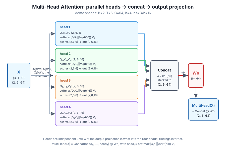
Here is the entire layer as one function. It takes the input $X$ and the four projection matrices $W_q, W_k, W_v, W_o$ (all (C, C)) plus the head count $h$, and walks the pipeline: project, split, per-head attention, concatenate, project. It returns the output and a cache of every intermediate so later lessons (and the exercises) can inspect the stages.

import numpy as np

def softmax(x, axis=-1):
    x = x - x.max(axis=axis, keepdims=True)   # subtract row max for stability
    e = np.exp(x)
    return e / e.sum(axis=axis, keepdims=True)

def multi_head_attention_forward(X, Wq, Wk, Wv, Wo, h):
    B, T, C = X.shape
    hs = C // h                                 # head size

    # 1. Project the full width, then split C into h heads and lift the head
    #    axis up front: (B, T, C) -> (B, T, h, hs) -> (B, h, T, hs)
    Q = (X @ Wq).reshape(B, T, h, hs).transpose(0, 2, 1, 3)
    K = (X @ Wk).reshape(B, T, h, hs).transpose(0, 2, 1, 3)
    V = (X @ Wv).reshape(B, T, h, hs).transpose(0, 2, 1, 3)

    # 2. Scaled dot-product attention, batched over BOTH B and h at once.
    #    Swap the LAST two axes of K: (B, h, T, hs) -> (B, h, hs, T)
    scores = Q @ K.transpose(0, 1, 3, 2) / np.sqrt(hs)   # (B, h, T, T)
    weights = softmax(scores, axis=-1)                    # (B, h, T, T)
    per_head = weights @ V                                 # (B, h, T, hs)

    # 3. Concatenate heads: (B, h, T, hs) -> (B, T, h, hs) -> (B, T, C)
    concat = per_head.transpose(0, 2, 1, 3).reshape(B, T, C)

    # 4. Output projection mixes the concatenated heads: (B, T, C) @ (C, C)
    out = concat @ Wo                                     # (B, T, C)

    cache = dict(Q=Q, K=K, V=V, scores=scores, weights=weights,
                 per_head=per_head, concat=concat, out=out)
    return out, cache

Notice how little there is. Two of the four steps, the split and the concat, are pure reshuffles with no math, and the attention itself is three lines identical to the single-head version except for the transpose axes. Now feed it a real batch and print the shape at every stage. We use the mini-GPT head configuration ($C = 64$, $h = 4$, so $hs = 16$) on a batch of two sequences of length six, with a default_rng(42) seed so the run is fully reproducible. We initialize the projections at scale 0.2 rather than the real-training 0.02 so the attention weights differentiate visibly instead of coming out nearly uniform.

rng = np.random.default_rng(42)
B, T, C, h = 2, 6, 64, 4
hs = C // h

X  = rng.standard_normal((B, T, C))       # unit-scale inputs
Wq = rng.standard_normal((C, C)) * 0.2    # 0.2 init so attention differentiates
Wk = rng.standard_normal((C, C)) * 0.2
Wv = rng.standard_normal((C, C)) * 0.2
Wo = rng.standard_normal((C, C)) * 0.2

out, cache = multi_head_attention_forward(X, Wq, Wk, Wv, Wo, h)

print("config: B=%d, T=%d, C=%d, h=%d, hs=%d" % (B, T, C, h, hs))
print("X                :", X.shape)
print("Q/K/V per head   :", cache["Q"].shape,       "(B, h, T, hs)")
print("scores           :", cache["scores"].shape,  "(B, h, T, T)")
print("weights          :", cache["weights"].shape, "(B, h, T, T)")
print("per-head output  :", cache["per_head"].shape,"(B, h, T, hs)")
print("concat           :", cache["concat"].shape,  "(B, T, C)")
print("final out        :", out.shape,              "(B, T, C)")

rowsums = cache["weights"].sum(axis=-1)   # (B, h, T)
print("attention rows all sum to 1?", np.allclose(rowsums, 1.0),
      " min=%.6f max=%.6f" % (rowsums.min(), rowsums.max()))

config: B=2, T=6, C=64, h=4, hs=16
X                : (2, 6, 64)
Q/K/V per head   : (2, 4, 6, 16) (B, h, T, hs)
scores           : (2, 4, 6, 6) (B, h, T, T)
weights          : (2, 4, 6, 6) (B, h, T, T)
per-head output  : (2, 4, 6, 16) (B, h, T, hs)
concat           : (2, 6, 64) (B, T, C)
final out        : (2, 6, 64) (B, T, C)
attention rows all sum to 1? True  min=1.000000 max=1.000000

Trace the shapes against the pipeline. $X$ came in at (2, 6, 64). After project-and-split, each of $Q, K, V$ is (2, 4, 6, 16), one (6, 16) head for every (batch, head) pair. The batched $Q K^\top$ produced scores of (2, 4, 6, 6), a full 6-by-6 attention table per head, and softmax left the weights the same shape with every row summing to 1 (confirmed: min and max row sums are both exactly 1.0). Multiplying by $V$ gave per-head outputs of (2, 4, 6, 16); the concat stacked the four heads back to (2, 6, 64); and $W_o$ returned the final output at (2, 6, 64), the identical shape we started with. The layer is shape-preserving, which is exactly what lets you stack many of them.

Reading the Heads: Different Patterns, Then Concatenated#

The shapes are right, but the point of multi-head attention is that the heads attend differently. Let us look at two of them and then confirm the concat really is just the heads stacked. This block reuses out, cache, hs, and h from above.

print("batch 0, head 0 weights (each row sums to 1):")
print(np.round(cache["weights"][0, 0], 3))
print("batch 0, head 1 weights (a DIFFERENT pattern, same positions):")
print(np.round(cache["weights"][0, 1], 3))

# The concat is EXACTLY the per-head outputs laid end to end.
per_head, concat = cache["per_head"], cache["concat"]
ok = all(np.allclose(concat[:, :, i*hs:(i+1)*hs], per_head[:, i, :, :])
         for i in range(h))
print("concat block i == head i output?", ok)
print("concat[0, 0, :4]   (start of head 0):", np.round(concat[0, 0, :4], 4))
print("per_head[0,0,0,:4] (head 0, pos 0)  :", np.round(per_head[0, 0, 0, :4], 4))

batch 0, head 0 weights (each row sums to 1):
[[0.005 0.008 0.002 0.972 0.001 0.012]
 [0.152 0.121 0.103 0.026 0.485 0.113]
 [0.    0.    0.007 0.991 0.    0.001]
 [0.448 0.24  0.013 0.    0.294 0.005]
 [0.539 0.015 0.169 0.009 0.247 0.022]
 [0.04  0.019 0.093 0.198 0.111 0.54 ]]
batch 0, head 1 weights (a DIFFERENT pattern, same positions):
[[0.282 0.105 0.018 0.073 0.003 0.519]
 [0.001 0.017 0.02  0.058 0.814 0.091]
 [0.029 0.018 0.802 0.113 0.037 0.   ]
 [0.033 0.119 0.244 0.06  0.054 0.49 ]
 [0.063 0.001 0.004 0.542 0.383 0.006]
 [0.145 0.153 0.501 0.088 0.068 0.044]]
concat block i == head i output? True
concat[0, 0, :4]   (start of head 0): [ 2.7813 -0.5535  1.2289 -0.1792]
per_head[0,0,0,:4] (head 0, pos 0)  : [ 2.7813 -0.5535  1.2289 -0.1792]

The two heads have learned to look at different things even though they see the same six positions. In head 0, position 0 pours 0.972 of its attention onto position 3; in head 1, that same position 0 splits its attention between position 5 (0.519) and position 0 (0.282), a completely different distribution. Every row in both tables still sums to 1, because softmax normalizes each head independently. This is the whole reason to have more than one head: each is a separate lens on the sequence.

The last check makes “concat” concrete. The first $hs = 16$ columns of the concatenated vector are byte-for-byte head 0’s output, concat[0, 0, :4] equals per_head[0, 0, 0, :4] exactly, and the same holds for every head’s block. Concatenation adds no arithmetic; it only decides the order in which the heads’ numbers sit in the final vector, which is precisely the order $W_o$ then reads them in.

Proving Wo Makes the Heads Interact#

The claim was that without $W_o$, heads stay isolated, and with it, they interact. That is testable. A full (C, C) $W_o$ lets every output dimension read all four heads; a block-diagonal $W_o$, one that is nonzero only within each head’s own 16-column block, can only ever mix dimensions inside a single head. If we knock out one head’s contribution and see how many output dimensions change, the two projections should behave very differently. This block reuses X, Wq, Wk, Wv, Wo, concat, out, C, hs, and h.

# A block-diagonal Wo: nonzero only within each head's own hs-block.
block_diag = np.zeros((C, C))
for i in range(h):
    s = slice(i*hs, (i+1)*hs)
    block_diag[s, s] = rng.standard_normal((hs, hs)) * 0.2
out_bd, _ = multi_head_attention_forward(X, Wq, Wk, Wv, block_diag, h)

# Zero out head 3's slice of the concat and see which output dims move.
concat_drop = concat.copy()
concat_drop[:, :, 3*hs:4*hs] = 0.0
moved_full = np.abs(concat_drop @ Wo - out)          # full Wo
moved_bd   = np.abs(concat_drop @ block_diag - out_bd)  # block-diagonal Wo

print("drop head 3 -> output dims changed (full Wo):      ",
      int((moved_full[0, 0] > 1e-9).sum()), "of", C)
print("drop head 3 -> output dims changed (block-diag Wo):",
      int((moved_bd[0, 0] > 1e-9).sum()), "of", C)

drop head 3 -> output dims changed (full Wo):       64 of 64
drop head 3 -> output dims changed (block-diag Wo): 16 of 64

The result is exactly the point of $W_o$ in one number. With the full projection, deleting a single head disturbs all 64 output dimensions: every output feature was reading from head 3 (among the others), so head 3 genuinely participates everywhere. With the block-diagonal projection, deleting head 3 changes only its own 16 dimensions, and the other three heads’ outputs are untouched, they never see head 3 at all. A block-diagonal $W_o$ reduces multi-head attention to four independent single-head layers glued side by side. The dense, learnable $W_o$ is the ingredient that turns four isolated lenses into one integrated representation, which is why it is a mandatory part of the layer and not an optional flourish.

Practice Exercises#

Try these before checking the hints. They reuse multi_head_attention_forward, softmax, and the seed-42 setup from the lesson.

Exercise 1: Rebuild the Concat With an Explicit Loop#

Prove to yourself that the transpose-then-reshape concat is equivalent to physically looping over heads and stacking their outputs. Take cache["per_head"] of shape (B, h, T, hs) and build the (B, T, C) concatenation by hand with np.concatenate, then confirm it matches cache["concat"].

# Your code here: build concat_manual from cache["per_head"] with a loop,
# then compare to cache["concat"]

Exercise 2: Confirm the Heads Are Truly Independent#

Run the layer, then re-run it after zeroing out head 2’s value projection columns, and confirm that only head 2’s slice of the concatenated output changes while the other heads’ slices are identical. This shows the per-head attention really is computed in isolation (before $W_o$).

# Your code here: compare cache["concat"] before and after zeroing the
# columns of Wv that feed head 2 (columns 2*hs to 3*hs), head by head

Exercise 3: Vary the Head Count at Fixed Width#

Multi-head attention lets you trade the number of heads against the head size while keeping $C$ fixed. For $C = 64$, run the layer with h in [1, 2, 4, 8] and print hs and the scores shape each time. Confirm the final output is always (B, T, 64) no matter how you slice the width.

# Your code here: loop over h in [1, 2, 4, 8], build fresh Wq/Wk/Wv/Wo,
# run the forward, print hs, cache["scores"].shape, and out.shape

Summary#

You assembled the complete multi-head attention forward pass: parallel per-head attention, concatenation, and the output projection that ties the heads together. Let’s review.

Key Concepts#

Parallel Attention Over the Head Axis

• With $Q, K, V$ shaped (B, h, T, hs), one @ computes every head’s attention at once; np.matmul batches over all leading axes, so the head axis behaves exactly like the batch axis
• Swap the last two axes of $K$ with K.transpose(0, 1, 3, 2) to get (B, h, hs, T); scores are (B, h, T, T), softmax runs over the last axis, and the per-head output is (B, h, T, hs)
• No Python loop over heads is needed, and none should be used

Concatenation

• The concat is the split in reverse: (B, h, T, hs) → transpose → (B, T, h, hs) → reshape → (B, T, C)
• It is pure memory reshuffling with no arithmetic; the first $hs$ columns are head 0’s output, the next $hs$ are head 1’s, verified byte-for-byte
• Always transpose before the reshape, or the vectors scramble silently

The Output Projection $W_o$

• $\text{MultiHead}(X) = \text{Concat}(head_1, \dots, head_h)\, W_o$, with $W_o$ a learned (C, C) matrix
• Because $W_o$ is dense, every output dimension reads all $C$ concatenated inputs, which is the only place the heads interact
• Proof: dropping one head with a full $W_o$ disturbs all 64 output dims; with a block-diagonal $W_o$ it disturbs only that head’s 16 dims, reducing the layer to independent single-head attentions

The Verified Forward

• Demo (seed 42, B=2, T=6, C=64, h=4, hs=16) flowed (2,6,64) → Q/K/V (2,4,6,16) → scores (2,4,6,6) → per-head (2,4,6,16) → concat (2,6,64) → out (2,6,64)
• Every attention row summed to 1 within each head, and two heads showed genuinely different attention distributions over the same positions

Why This Matters#

Multi-head attention is the layer at the center of every transformer block, and you now have its forward pass in full, not as a diagram but as a function you ran and inspected. The two ideas that make it work are worth carrying forward. The first is that parallelism over heads is free in NumPy: because matrix multiplication batches over leading axes, “run $h$ attentions” is the same code as “run one attention” with an extra axis, which is exactly why transformers are so efficient on modern hardware. The second is that the output projection is not decoration. You proved, with a block-diagonal counterexample, that without $W_o$ the heads are strangers; $W_o$ is what lets a model combine “what rhymes” and “what is the subject” into a single learned feature. When you later read that a transformer has $h$ heads and a c_proj or out_proj matrix, you will know precisely what each does and why removing either would break the layer.

You also now hold every shape in the pipeline. That fluency, knowing that scores are (B, h, T, T) and the concat is (B, T, C) without pausing to derive it, is what makes the backward pass tractable. A gradient has the same shape as the thing it belongs to, so once the forward shapes are second nature, the backward pass becomes a matter of routing gradients through the same axes in reverse.

Continue Building Your Skills#

You can now run the entire multi-head attention forward pass, from projecting $X$ into $h$ heads all the way to the mixed output that $W_o$ produces. Everything so far has flowed forward. The next lesson turns the pipeline around and derives the backward pass through multi-head attention: how a gradient arriving at the output flows back through $W_o$, un-concatenates into per-head gradients, threads back through each head’s scaled dot-product attention (reusing the single-head gradients from Module 2, named dQuery, dKey, dValue to keep the query/key/value gradients distinct and deploy-safe), and finally recombines across the split to give the gradients on $W_q, W_k, W_v$. You will assemble it step by step and verify the whole thing against a numerical gradient, exactly as you did for the single head, so that by the end you can trust every number your multi-head layer produces in both directions.