Lesson 4 - The Multi-Head Backward Pass

Welcome to The Multi-Head Backward Pass#

In Lesson 3 you built the full forward pass of multi-head attention: project the input into a query, key, and value with three (C, C) matrices; split each into h heads of size hs = C / h; run scaled dot-product attention in every head at once; concatenate the head outputs back into a single (B, T, C) tensor; and mix them with an output projection Wo. That gives you out, but a forward pass alone cannot train anything. To learn Wq, Wk, Wv, and Wo, gradient descent needs the gradient of the loss with respect to each of them, and with respect to the input X so the layers below can train too. This lesson derives that backward pass end to end and, as always in this course, proves it is correct with a numerical gradient check.

The good news is that you already did the genuinely hard part in Module 2. The backward pass through a single scaled dot-product attention head, including the subtle softmax Jacobian, is done. Multi-head attention wraps that head in three new operations: an output projection, a split, and a concatenation. So the whole job here is to differentiate those three wrappers and then reuse the single-head backward, this time batched over the head axis instead of run once. The split and the concat are pure reshapes and transposes, and the gradient of a reshape is just the inverse reshape. Get the axis bookkeeping right and the numbers fall into place.

By the end of this lesson, you will be able to:

• Cache the multi-head forward pass so the backward pass has every tensor it needs
• Differentiate the output projection to get dWo and dconcat
• Split dconcat back into per-head dheadout (the inverse of the forward split)
• Run the single-head attention backward batched over the head axis to get dValue, dscores, dQuery, and dKey
• Merge the per-head gradients back to (B, T, C) and finish at dWq, dWk, dWv, and dX
• Verify every gradient against a float64 finite-difference estimate and read a real max relative error

You should be comfortable with the multi-head forward from Lesson 3 and with the single-head attention backward from Module 2. Let’s begin.

Setup: A Tiny Multi-Head Layer in float64#

To prove gradients numerically we want dimensions small enough that a finite-difference check over every entry runs instantly, and float64 so the check has the precision to trust. We use a batch of B = 2, sequence length T = 4, model width C = 8, and h = 2 heads, which makes the head size hs = C / h = 4. Everything is seeded so the run is fully reproducible.

The forward pass is exactly the Lesson 3 code, rewritten to return a cache of the tensors the backward pass will reuse. The two reshape helpers, split_heads and merge_heads, are the same ones from the forward lesson: split_heads turns (B, T, C) into (B, h, T, hs), and merge_heads is its exact inverse.

import numpy as np

np.random.seed(42)
B, T, C, h = 2, 4, 8, 2
hs = C // h                      # 4: head size

def softmax(x, axis=-1):
    x = x - x.max(axis=axis, keepdims=True)   # stable: subtract row max
    e = np.exp(x)
    return e / e.sum(axis=axis, keepdims=True)

# float64 everywhere (default), small init
X  = np.random.randn(B, T, C) * 0.5
Wq = np.random.randn(C, C) * 0.1
Wk = np.random.randn(C, C) * 0.1
Wv = np.random.randn(C, C) * 0.1
Wo = np.random.randn(C, C) * 0.1
G  = np.random.randn(B, T, C)    # fixed random output directions (defines the loss)

def split_heads(M):
    # (B, T, C) -> (B, T, h, hs) -> (B, h, T, hs)
    return M.reshape(B, T, h, hs).transpose(0, 2, 1, 3)

def merge_heads(M):
    # (B, h, T, hs) -> (B, T, h, hs) -> (B, T, C)   (inverse of split_heads)
    return M.transpose(0, 2, 1, 3).reshape(B, T, C)

def mha_forward(X, Wq, Wk, Wv, Wo):
    Q = split_heads(X @ Wq)                              # (B, h, T, hs)
    K = split_heads(X @ Wk)                              # (B, h, T, hs)
    V = split_heads(X @ Wv)                              # (B, h, T, hs)
    scores = Q @ K.transpose(0, 1, 3, 2) / np.sqrt(hs)  # (B, h, T, T)
    Aweights = softmax(scores, axis=-1)                 # (B, h, T, T)
    headout = Aweights @ V                              # (B, h, T, hs)
    concat = merge_heads(headout)                       # (B, T, C)
    out = concat @ Wo                                   # (B, T, C)
    cache = (X, Wq, Wk, Wv, Wo, Q, K, V, Aweights, concat)
    return out, cache

out, cache = mha_forward(X, Wq, Wk, Wv, Wo)
print("X:", X.shape, " out:", out.shape, " dtype:", out.dtype)
print("split Q:", cache[5].shape, " scores/Aweights:", cache[8].shape)

X: (2, 4, 8)  out: (2, 4, 8)  dtype: float64
split Q: (2, 2, 4, 4)  scores/Aweights: (2, 2, 4, 4)

The layer maps (2, 4, 8) to (2, 4, 8). Inside, Q, K, V live in the four-axis head layout (2, 2, 4, 4) = (B, h, T, hs), and each head’s attention weights Aweights are (B, h, T, T). The cache tuple carries the ten tensors the backward pass differentiates against, including Aweights for the softmax step and concat for the output projection.

A Scalar Loss So dout Is Known#

Backpropagation starts from a scalar. In the finished GPT that scalar is the cross-entropy loss many layers downstream, but to isolate and test just this layer we invent the simplest scalar whose gradient with respect to out we can write by hand. Take a fixed random tensor $G$ the same shape as out and define

Because $L$ is a plain sum of out weighted by the constants $G$, its derivative with respect to each entry of out is exactly the matching entry of $G$. So the upstream gradient entering the layer is simply dout = G, with no chain rule needed. This is the standard trick for unit-testing a layer: choose a loss whose dout you know exactly, then check everything the layer derives from it.

def loss_from_out(out):
    return np.sum(out * G)          # scalar; dL/dout is therefore exactly G

L = loss_from_out(out)
dout = G                            # upstream gradient dL/dout
print("L:", round(float(L), 6), " dout:", dout.shape)

L: 0.021531  dout: (2, 4, 8)

We keep the course convention that a name like dX means $\partial L / \partial X$, the gradient of the loss with respect to X, and it always has the same shape as X. That shape rule is your first defense against transpose bugs: if a gradient comes out shaped differently from its quantity, something is wrong before you ever run the numerical check.

One naming note carried from Module 2, and it matters here too: the gradients of the query, key, and value tensors are written dQuery, dKey, dValue, never abbreviated. The forward variables stay Q, K, V, and the weight gradients stay dWq, dWk, dWv, dWo, which are already unambiguous. Keeping the projected-tensor gradients spelled out keeps the derivation readable and consistent across every lesson.

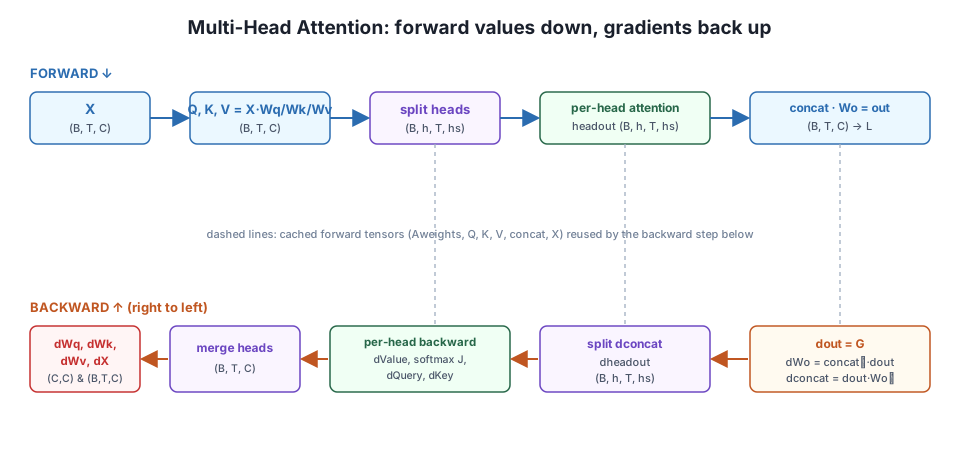
That picture is the whole lesson on one page. Now we derive each backward arrow, right to left, in the exact order the code runs.

Step 1: Through the Output Projection, dWo and dconcat#

The last forward operation was out = concat @ Wo, an ordinary matrix multiply of concat shaped (B, T, C) by the shared weight Wo shaped (C, C). This is the same dense-layer gradient rule from the foundations course, applied with concat playing the role of the layer input. Wo is shared across the batch, so its gradient sums the per-item contributions; dconcat flows straight back with Wo transposed:

For dWo, each batch element contributes concat[b].T @ dout[b] of shape (C, C), and summing over the batch axis collapses those into one (C, C) gradient matching Wo. The batched transpose swaps the last two axes with concat.transpose(0, 2, 1), not concat.T (which would also flip the batch axis and give the wrong shape).

dWo = np.sum(concat.transpose(0, 2, 1) @ dout, axis=0)   # (C, C)
dconcat = dout @ Wo.T                                     # (B, T, C)

Check the shapes: concat.transpose(0, 2, 1) is (B, C, T) and dout is (B, T, C), so the per-batch product is (B, C, C), and the sum over the batch axis gives (C, C) to match Wo. And dout (B, T, C) times Wo.T (C, C) broadcasts over the batch to (B, T, C), matching concat. dWo is a finished parameter gradient; dconcat is the signal we now feed back through the concatenation.

Step 2: Split the Gradient Back Into Heads, dheadout#

The forward pass built concat from the per-head outputs with merge_heads, which reshaped (B, h, T, hs) into (B, T, C). That operation only rearranges numbers; it does not add, multiply, or combine them. The gradient of a pure rearrangement is the same rearrangement run in reverse. So to push dconcat back into the head layout, we apply the inverse of merge_heads, which is exactly split_heads:

dheadout = split_heads(dconcat)   # (B, h, T, hs)

Every entry of dconcat lands back on the head and position it came from in the forward split, because split_heads and merge_heads are exact inverses. dheadout is now the gradient of the loss with respect to each head’s output headout, laid out (B, h, T, hs), ready to enter the per-head attention backward.

Step 3: The Per-Head Attention Backward, Batched Over Heads#

Here is the payoff for all the work in Module 2. Each head ran the identical scaled dot-product attention headout = Aweights @ V with Aweights = softmax(Q Kᵀ / √hs), and you already derived that backward pass. The only change is that the head is no longer run once on a (B, T, ...) tensor; it runs across the head axis on a (B, h, T, ...) tensor. NumPy’s batched matrix multiply treats every axis but the last two as a batch, so the exact same lines work unchanged, we just transpose the last two axes with transpose(0, 1, 3, 2) instead of transpose(0, 2, 1).

Start at the value multiply headout = Aweights @ V. By the matrix-multiply rule, the gradient on each factor is the incoming gradient times the other factor, transposed on its last two axes:

dAweights = dheadout @ V.transpose(0, 1, 3, 2)         # (B, h, T, T)
dValue = Aweights.transpose(0, 1, 3, 2) @ dheadout     # (B, h, T, hs)

Next, the softmax. Each row of Aweights is a softmax over the last axis, so its gradient uses the softmax Jacobian $\operatorname{diag}(A) - A A^\top$, which in vectorized form is each probability times its own incoming gradient minus the row-probability-weighted average of the incoming gradients:

The keepdims=True sum runs over the last axis, so it broadcasts correctly across all B and h rows at once. Then divide by $\sqrt{hs}$ to undo the forward scale, which is a constant and passes straight through:

dscores = Aweights * (dAweights - np.sum(dAweights * Aweights, axis=-1, keepdims=True))
dscores = dscores / np.sqrt(hs)                        # (B, h, T, T)

Finally, the score matrix scores_raw = Q @ Kᵀ. The matrix-multiply rule again, with the batched last-two-axes transpose:

dQuery = dscores @ K                        # (B, h, T, hs)
dKey = dscores.transpose(0, 1, 3, 2) @ Q    # (B, h, T, hs)

Watch the transpose axes carefully: with a four-axis tensor the batched transpose is transpose(0, 1, 3, 2), which swaps only T and the last axis while leaving B and h in place. Using transpose(0, 2, 1) here (the three-axis version from Module 2) would be a bug, and the gradient check would catch it immediately. We now hold dQuery, dKey, and dValue, each (B, h, T, hs), the gradients on the three projected tensors in their per-head layout.

Step 4: Merge the Heads, Then Back to dWq, dWk, dWv, dX#

dQuery, dKey, and dValue are in the four-axis head layout, but the projections that produced them, Q = X @ Wq and friends, operated on the merged (B, T, C) tensors before the split. To continue we must undo that split, which, by the same reshape-inverse logic as Step 2, means applying merge_heads:

dQm = merge_heads(dQuery)   # (B, T, C)
dKm = merge_heads(dKey)     # (B, T, C)
dVm = merge_heads(dValue)   # (B, T, C)

Now we are back to (B, T, C) gradients on the projected tensors, exactly the situation from the single-head Module 2 lesson. Each projection is a matrix multiply of X (B, T, C) by a shared weight (C, C), so the weight gradient sums per-batch contributions and the input gradient adds over the three projection paths:

dWq = np.sum(X.transpose(0, 2, 1) @ dQm, axis=0)   # (C, C)
dWk = np.sum(X.transpose(0, 2, 1) @ dKm, axis=0)   # (C, C)
dWv = np.sum(X.transpose(0, 2, 1) @ dVm, axis=0)   # (C, C)

dX = dQm @ Wq.T + dKm @ Wk.T + dVm @ Wv.T          # (B, T, C)

X feeds all three projections, so gradient flows back to it along three routes and they add, the multivariate chain rule. Collect the whole backward pass into one function and confirm every gradient has the shape of the quantity it belongs to.

def mha_backward(dout, cache):
    X, Wq, Wk, Wv, Wo, Q, K, V, Aweights, concat = cache

    # output projection
    dWo = np.sum(concat.transpose(0, 2, 1) @ dout, axis=0)   # (C, C)
    dconcat = dout @ Wo.T                                    # (B, T, C)

    # split gradient back into heads (inverse of the forward concat)
    dheadout = split_heads(dconcat)                          # (B, h, T, hs)

    # per-head attention backward, batched over B and h
    dAweights = dheadout @ V.transpose(0, 1, 3, 2)           # (B, h, T, T)
    dValue = Aweights.transpose(0, 1, 3, 2) @ dheadout       # (B, h, T, hs)

    dscores = Aweights * (dAweights - np.sum(dAweights * Aweights, axis=-1, keepdims=True))
    dscores = dscores / np.sqrt(hs)                          # (B, h, T, T)

    dQuery = dscores @ K                                     # (B, h, T, hs)
    dKey = dscores.transpose(0, 1, 3, 2) @ Q                 # (B, h, T, hs)

    # merge heads back to (B, T, C) (inverse of the forward split)
    dQm = merge_heads(dQuery)
    dKm = merge_heads(dKey)
    dVm = merge_heads(dValue)

    dWq = np.sum(X.transpose(0, 2, 1) @ dQm, axis=0)         # (C, C)
    dWk = np.sum(X.transpose(0, 2, 1) @ dKm, axis=0)         # (C, C)
    dWv = np.sum(X.transpose(0, 2, 1) @ dVm, axis=0)         # (C, C)

    dX = dQm @ Wq.T + dKm @ Wk.T + dVm @ Wv.T                # (B, T, C)
    return dWq, dWk, dWv, dWo, dX

dWq, dWk, dWv, dWo, dX = mha_backward(dout, cache)
print("dWq:", dWq.shape, " dWk:", dWk.shape, " dWv:", dWv.shape, " dWo:", dWo.shape)
print("dX:", dX.shape)

dWq: (8, 8)  dWk: (8, 8)  dWv: (8, 8)  dWo: (8, 8)
dX: (2, 4, 8)

Every parameter gradient is (C, C) = (8, 8), matching its weight, and dX is (2, 4, 8), matching the input. The shapes are right, but shapes only prove the plumbing lines up, not that the numbers are correct. For that we need the gradient check.

Proving It: A Numerical Gradient Check#

The definition of a derivative gives a way to estimate any gradient with no calculus at all: nudge one number up by a tiny $\epsilon$, nudge it down by $\epsilon$, see how much the loss $L$ moved, and divide. This central finite difference is accurate to order $\epsilon^2$:

If the analytic backward pass is correct, the numerical estimate must agree with it for every entry of every parameter and of X. We measure agreement with the max relative error: the largest, across the tensor, of $|a - n| \, / \, \max(|a|, |n|)$, where $a$ is analytic and $n$ is numerical. In float64 with $\epsilon = 10^{-5}$, a correct gradient lands around $10^{-6}$ or smaller; anything like $10^{-2}$ means a real bug.

def numerical_grad(param):
    eps = 1e-5
    grad = np.zeros_like(param)
    it = np.nditer(param, flags=["multi_index"])
    while not it.finished:
        idx = it.multi_index
        original = param[idx]
        param[idx] = original + eps
        Lp = loss_from_out(mha_forward(X, Wq, Wk, Wv, Wo)[0])
        param[idx] = original - eps
        Lm = loss_from_out(mha_forward(X, Wq, Wk, Wv, Wo)[0])
        param[idx] = original          # always restore the entry
        grad[idx] = (Lp - Lm) / (2 * eps)
        it.iternext()
    return grad

def max_rel_err(analytic, numeric):
    denom = np.maximum(np.abs(analytic), np.abs(numeric)) + 1e-12
    return np.max(np.abs(analytic - numeric) / denom)

print("max relative error (analytic vs. numerical):")
print("  dWq:", max_rel_err(dWq, numerical_grad(Wq)))
print("  dWk:", max_rel_err(dWk, numerical_grad(Wk)))
print("  dWv:", max_rel_err(dWv, numerical_grad(Wv)))
print("  dWo:", max_rel_err(dWo, numerical_grad(Wo)))
print("  dX :", max_rel_err(dX,  numerical_grad(X)))

max relative error (analytic vs. numerical):
  dWq: 1.1258458882596268e-07
  dWk: 8.349931940877706e-09
  dWv: 2.7289366668444704e-10
  dWo: 2.3034316001555859e-10
  dX : 2.4085590689416927e-09

Every error sits between $10^{-7}$ and $10^{-10}$, far below the $10^{-4}$ threshold that separates “correct” from “buggy.” That is the proof: the analytic backward pass, split, batched softmax Jacobian, merge, and all, computes the same gradients that a brute-force perturbation of the loss produces. Run the whole script a second time and the numbers are byte-for-byte identical, because the seed fixes every random draw and the finite-difference loop is deterministic. dWo and dValue’s path are smallest because they flow through the fewest nonlinear steps; dWq is largest because its gradient passes through the full softmax coupling in every head, yet even it is essentially perfect.

Practice Exercises#

Try these before checking the hints. They reuse mha_forward, mha_backward, loss_from_out, numerical_grad, split_heads, merge_heads, and the tensors defined above.

Exercise 1: Prove Split and Merge Are Exact Inverses#

The whole backward pass leans on merge_heads and split_heads being perfect inverses of each other. Confirm it directly: take a random (B, T, C) tensor, split it and merge it back, and check you recover the original exactly; then do the round trip the other way starting from a (B, h, T, hs) tensor.

Z = np.random.randn(B, T, C)
# Your code here: verify merge_heads(split_heads(Z)) == Z, and the reverse round trip

Exercise 2: Break the Four-Axis Transpose on Purpose#

Copy mha_backward into broken_backward and change only the dKey line to use the three-axis transpose dscores.transpose(0, 2, 1) instead of dscores.transpose(0, 1, 3, 2). Run it, take its dWk, and gradient-check that one gradient. Watch the error explode, then restore the correct axes.

# Your code here: copy mha_backward, break only the dKey transpose axes,
# recompute dWk, and print max_rel_err(dWk_wrong, numerical_grad(Wk))

Exercise 3: Confirm the Heads Are Independent Before the Merge#

Inside a single head, attention never looks at the other heads; they only mix in the output projection Wo. Verify this in the backward pass: zero out the incoming gradient for head 0 only (set dheadout[:, 0] = 0) and confirm that dValue, dscores, and dQuery for head 1 are completely unchanged, while head 0’s are now zero.

# Your code here: run the per-head backward with dheadout, then again with
# dheadout_masked (head 0 zeroed), and compare the two heads' dQuery

Summary#

You derived and verified the complete backward pass through multi-head attention, the last piece of machinery before you can package the whole thing into a trainable layer. Let’s review.

Key Concepts#

The Setup

• Cache the forward tensors (X, Wq, Wk, Wv, Wo, Q, K, V, Aweights, concat) so the backward pass can reuse them
• Use tiny dims (B=2, T=4, C=8, h=2, hs=4) and float64 so a finite-difference check is fast and trustworthy
• Define a scalar loss $L = \sum \text{out} \cdot G$ so the upstream gradient is exactly dout = G

The Backward Pass, In Order

• dWo = sum over batch of concatᵀ @ dout, dconcat = dout @ Woᵀ — the output projection, a shared-weight dense layer
• dheadout = split_heads(dconcat) — the gradient of the concat is the inverse reshape (the split)
• Per head, batched over the head axis: dAweights = dheadout @ Vᵀ, dValue = Aweightsᵀ @ dheadout; softmax Jacobian dscores = Aweights * (dAweights - sum(dAweights*Aweights, axis=-1, keepdims)); dscores /= sqrt(hs); dQuery = dscores @ K, dKey = dscoresᵀ @ Q — all with the four-axis transpose transpose(0, 1, 3, 2)
• dQm, dKm, dVm = merge_heads(dQuery/dKey/dValue) — the gradient of the split is the inverse reshape (the merge)
• dWq/dWk/dWv = sum over batch of Xᵀ @ dQm/dKm/dVm, and dX = dQm @ Wqᵀ + dKm @ Wkᵀ + dVm @ Wvᵀ — three projection paths add at the input

Proving It

• Every gradient has the same shape as its quantity; a shape mismatch is a bug you can catch before running
• A central finite difference $(L(\theta+\epsilon) - L(\theta-\epsilon)) / 2\epsilon$ estimates any gradient with no calculus
• Real max relative errors were 1e-7 (dWq) down to 1e-10 (dWo, dWv), all far below the 1e-4 bar, and identical on re-run

Why This Matters#

Multi-head attention is where a transformer does most of its representational work, and until this lesson you could only run it forward. Now you can train it. The striking lesson of the derivation is how little new mathematics multi-head attention needed: the output projection is an ordinary dense layer you already knew, the split and concat are reshapes whose gradients are just their own inverses, and the attention math itself is Module 2’s single-head backward run unchanged across a head axis. Complex-looking architectures are almost always assemblies of a few simple, well-understood gradient rules, and the skill that matters is decomposing them cleanly and keeping the axis bookkeeping straight.

Just as important, you proved it. A wrong gradient does not crash; it quietly trains the wrong model, and in a layer with a split, a batched softmax, and a merge there are many places for a transpose to go silently wrong. The perturb-and-compare gradient check is the professional standard for verifying any custom layer, and reading a max relative error of 1e-7 is the difference between hoping your attention layer is correct and knowing it is.

Continue Building Your Skills#

You now have every gradient for a full multi-head attention layer, derived by hand and confirmed against the numerical truth, split and merge included. What remains is to package it. In the next lesson, the module’s guided project, you will fold this forward and backward pass into one reusable MultiHeadAttention layer class with forward and backward methods, an object that owns its own Wq, Wk, Wv, and Wo, stashes its cache during the forward call, and hands back dWq, dWk, dWv, dWo, and dX during the backward call, gradient-checked end to end. That class is the attention block you will drop into the full transformer layer, wiring it together with the residual connections, layer norm, and feed-forward network in the modules ahead. The hard derivation is behind you; from here on, multi-head attention is a component you can build once and trust.