Lesson 1 - Why Attention Needs Position

Welcome to Why Attention Needs Position#

Across the last three modules you built a working attention head from scratch: you projected the input into queries, keys, and values, scored every query against every key, softmaxed those scores into weights, and mixed the values. You even ran several heads in parallel. That machinery is the engine of the tiny character-level GPT you are assembling. But it has a blind spot so fundamental that it is easy to miss, and this module exists entirely to fix it.

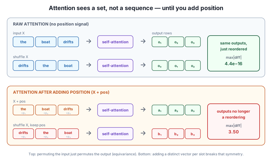
Here is the blind spot in one sentence: raw self-attention has no idea what order its inputs came in. It reads a sequence the way you would read a pile of loose word-cards dumped on a table, as a set, not a line of text. To attention, “the boat drifts” and “drifts boat the” carry the same information. For a model that is supposed to predict the next character of English, that is a disaster: word order is most of what meaning is. Before we can train the GPT, we have to hand attention a sense of position on purpose.

By the end of this lesson, you will be able to:

• Explain what it means for self-attention to be permutation-equivariant (and why people also call it permutation-invariant)
• Show in NumPy that permuting the input positions permutes the output identically, with a max difference near machine zero
• Connect this to something you already saw: identical tokens producing identical attention rows because there was no position signal
• Explain why position information must be added to the token representations before attention, not bolted on after
• Preview the three pieces this module builds: token embeddings, sinusoidal positional encoding, and learned positional embeddings

You should be comfortable with the single-head forward pass from Module 2 and with NumPy indexing and matrix multiplication. Let’s find the blind spot and then close it.

Attention Reads a Set, Not a Sequence#

Recall the shape of one self-attention head. Activations flow as $(B, T, C)$: batch $B$, sequence length $T$, model width $C$. The head projects the input $X$ into three $(B, T, hs)$ tensors, scores them, softmaxes, and mixes:

Look closely at where position could possibly enter. The projections $X W_q, X W_k, X W_v$ act on each row of $X$ independently, the same weight matrix applied to position 0, position 1, and position 5 alike. The score between query $i$ and key $j$ depends only on the contents of rows $i$ and $j$, never on how far apart $i$ and $j$ are or which one comes first. Nothing in the formula knows that row 2 sits between row 1 and row 3. The only thing distinguishing one position from another is whatever happens to be in its vector, and right now that vector is pure token content with no positional stamp.

That property has a precise name. Self-attention is permutation-equivariant: if you shuffle the input rows with some permutation, the output rows come out shuffled by the exact same permutation, and nothing else changes. Written compactly, for any permutation $P$ of the $T$ positions:

People often say attention is permutation-invariant, and for a good reason: the set of output vectors is unchanged by the shuffle, only their order moves. Either way the message is the same, attention carries no built-in notion of order. The order has to come from the vectors themselves.

Proving Permutation Equivariance in NumPy#

Talk is cheap; let’s make attention betray itself. We will take a small input $X$ of shape $(1, 6, 8)$, run it through a self-attention head, and then run a shuffled copy of $X$ through the same head. If attention is equivariant, the shuffled run’s output must equal the original output with its rows shuffled the same way, down to floating-point noise.

We use the canonical softmax and single-head forward pass from Module 2, and seed everything with 42 so the run is fully reproducible. The projection matrices use a demo init of * 0.5 so the attention weights are not washed out to uniform; the exact scale does not matter here, equivariance holds for any weights.

import numpy as np

def softmax(x, axis=-1):
    x = x - x.max(axis=axis, keepdims=True)   # subtract row max for stability
    e = np.exp(x)
    return e / e.sum(axis=axis, keepdims=True)

def self_attention(X, Wq, Wk, Wv):
    # X: (B, T, C);  Wq/Wk/Wv: (C, hs)
    Q, K, V = X @ Wq, X @ Wk, X @ Wv          # each (B, T, hs)
    hs = Q.shape[-1]
    scores = Q @ K.transpose(0, 2, 1) / np.sqrt(hs)   # (B, T, T)
    weights = softmax(scores, axis=-1)         # (B, T, T)
    return weights @ V                         # out: (B, T, hs)

np.random.seed(42)
B, T, C = 1, 6, 8
X  = np.random.randn(B, T, C)
Wq = np.random.randn(C, C) * 0.5
Wk = np.random.randn(C, C) * 0.5
Wv = np.random.randn(C, C) * 0.5

# a permutation of the T = 6 positions
perm = np.array([3, 0, 5, 1, 4, 2])

out      = self_attention(X, Wq, Wk, Wv)               # attend, then reorder rows
out_perm = self_attention(X[:, perm, :], Wq, Wk, Wv)   # reorder rows, then attend

max_diff = np.abs(out_perm - out[:, perm, :]).max()
print("out shape:", out.shape)
print("max |attn(X[perm]) - attn(X)[perm]| =", max_diff)

The key line is the comparison. out[:, perm, :] takes the original output and shuffles its rows by perm. out_perm shuffles the input first and then attends. Equivariance predicts these two are identical.

out shape: (1, 6, 8)
max |attn(X[perm]) - attn(X)[perm]| = 4.440892098500626e-16

The maximum absolute difference is about $4.4 \times 10^{-16}$, which is machine epsilon for float64, not a real difference at all, just the last bit of floating-point rounding. Run the block a second time and you get the identical number; there is no randomness left after the seed. Attention genuinely cannot tell the shuffled input from the original: it produced the same six output vectors, only reordered. Order was never part of the computation.

The Symptom You Already Saw: Identical Tokens, Identical Rows#

This blind spot is not new; you brushed against it back in Module 1. When two positions in a sequence held the same token vector, they produced the same attention output, byte for byte. At the time that looked like a quirk. Now you can name it: with no position signal, two positions that carry identical content are literally indistinguishable to attention, so of course they get identical outputs.

Let’s confirm it directly. We place the same token vector at position 0 and position 4 of a sequence, run attention, and compare those two output rows.

import numpy as np

def softmax(x, axis=-1):
    x = x - x.max(axis=axis, keepdims=True)
    e = np.exp(x)
    return e / e.sum(axis=axis, keepdims=True)

def self_attention(X, Wq, Wk, Wv):
    Q, K, V = X @ Wq, X @ Wk, X @ Wv
    hs = Q.shape[-1]
    scores = Q @ K.transpose(0, 2, 1) / np.sqrt(hs)
    weights = softmax(scores, axis=-1)
    return weights @ V

np.random.seed(42)
C = 8
Wq = np.random.randn(C, C) * 0.5
Wk = np.random.randn(C, C) * 0.5
Wv = np.random.randn(C, C) * 0.5

X = np.random.randn(1, 6, C)
tok = np.random.randn(C)     # one token vector
X[0, 0, :] = tok             # place it at position 0
X[0, 4, :] = tok             # and the identical vector at position 4

out = self_attention(X, Wq, Wk, Wv)
print("rows 0 and 4 identical? ", np.allclose(out[0, 0], out[0, 4]))
print("max |out[0] - out[4]| =", np.abs(out[0, 0] - out[0, 4]).max())

rows 0 and 4 identical?  True
max |out[0] - out[4]| = 0.0

Exactly zero. Position 0 and position 4 hold the same content, and because attention has no way to factor in “you are near the start” versus “you are further along,” it hands them the same answer. In real language that is wrong: the first “the” in a sentence and a later “the” play different grammatical roles, and a good model must be able to treat them differently. It cannot, as long as their vectors are identical. The fix has to make those two vectors different according to where they sit.

Breaking the Symmetry: Add Position#

So we cannot get order out of attention unless we put it into the vectors first. The plan is simple and is exactly what real transformers do: before attention, add a distinct vector to each position. If position 0 gets one offset and position 4 gets a different offset, then the two “the” tokens above stop being identical, their query and key vectors diverge, and attention can finally tell them apart.

To show that adding position genuinely breaks the equivariance, we repeat the shuffle experiment, but this time we add a per-slot vector pos before attending. Here pos[t] is just a different constant for each position slot $t$; it is a stand-in for the real positional encodings you build later in this module. The important move is that when we shuffle the tokens, the position vectors stay in their slots, position 0 always gets pos[0], no matter which token lands there.

import numpy as np

def softmax(x, axis=-1):
    x = x - x.max(axis=axis, keepdims=True)
    e = np.exp(x)
    return e / e.sum(axis=axis, keepdims=True)

def self_attention(X, Wq, Wk, Wv):
    Q, K, V = X @ Wq, X @ Wk, X @ Wv
    hs = Q.shape[-1]
    scores = Q @ K.transpose(0, 2, 1) / np.sqrt(hs)
    weights = softmax(scores, axis=-1)
    return weights @ V

np.random.seed(42)
B, T, C = 1, 6, 8
X  = np.random.randn(B, T, C)
Wq = np.random.randn(C, C) * 0.5
Wk = np.random.randn(C, C) * 0.5
Wv = np.random.randn(C, C) * 0.5
perm = np.array([3, 0, 5, 1, 4, 2])

# a distinct vector per position slot (a stand-in for real positional encoding)
pos = np.zeros((B, T, C))
for t in range(T):
    pos[0, t, :] = 0.6 * (t + 1)

Xp      = X + pos                      # tokens in order, with position
Xp_perm = X[:, perm, :] + pos          # tokens shuffled, position slots unchanged

outp      = self_attention(Xp, Wq, Wk, Wv)
outp_perm = self_attention(Xp_perm, Wq, Wk, Wv)

max_diff = np.abs(outp_perm - outp[:, perm, :]).max()
print("max |attn(shuffle + pos) - attn(with pos)[perm]| =", max_diff)

max |attn(shuffle + pos) - attn(with pos)[perm]| = 3.499757764020842

The maximum difference jumps from $4.4 \times 10^{-16}$ (indistinguishable) to about 3.50 (wildly different). Adding position did exactly what we wanted: the shuffled run is no longer a simple reordering of the original. Attention now notices that the tokens moved, because moving a token changes which position vector it is paired with, which changes its query and key, which changes every score it participates in. Rerun the block and you get the same 3.50; the whole thing is deterministic under the seed.

That single number is the entire justification for the rest of this module. Attention with no position is order-blind (difference $\approx 0$); attention with position added is order-aware (difference $\approx 3.5$). Everything from here is about what vector to add.

Where Position Has To Go#

One design choice deserves a word, because it surprises people: we add the position vector to the token vector rather than, say, concatenating a position index onto each row. Both are possible, but real transformers add, and there is a clean reason. The token embedding and the positional encoding live in the same $C$-dimensional space, so their sum is still a $C$-vector that flows through the unchanged $(B, T, C)$ pipeline. The projections $W_q, W_k, W_v$ then get to learn how to read the mixture, pulling out “what token is this” and “where is it” as the training signal demands. Adding keeps the width fixed and lets the model sort out the blend; concatenating would grow $C$ and force you to decide the split up front.

There is also a subtlety worth flagging for later. Adding the same position vector everywhere would do nothing, it has to be distinct per position to break the symmetry, which our 0.6 * (t + 1) toy satisfied. But a good positional signal needs more than distinctness: it should let the model reason about relative distance (“three tokens back”), extend to sequences longer than any it trained on, and not blow up in magnitude. Our crude linear ramp fails several of those. Designing a position vector that does all of it well is precisely the job of the sinusoidal and learned encodings coming up.

Practice Exercises#

Try these before checking the hints. They reuse the softmax and self_attention functions and the seed-42 setup from above.

Exercise 1: Forget To Reorder the Right-Hand Side#

Take the Part 1 setup (no position). Instead of comparing out_perm against out[:, perm, :], compare it against the unshuffled out with no reorder: compute np.abs(out_perm - out).max(). Explain in a comment why this number is large even though attention is equivariant.

# Your code here: reuse X, Wq, Wk, Wv, perm, out, out_perm from Part 1

Exercise 2: A Constant Offset Does Nothing#

In the Part 2 code, replace the per-slot pos with the same vector at every position, for example pos[0, t, :] = 0.6 for all t (drop the t + 1). Re-run the shuffle comparison and report the new max difference. Explain why it collapses back toward zero.

# Your code here: same as Part 2 but with a constant (position-independent) offset

Exercise 3: Distinguish the Two Identical “the” Tokens#

Return to the identical-tokens demo where positions 0 and 4 held the same vector tok and produced identical output rows. Add the per-slot pos (from Part 2) to X before attending, then re-check whether output rows 0 and 4 are still identical.

# Your code here: X[0,0]=tok; X[0,4]=tok; then attend to (X + pos)

Summary#

You found the blind spot at the heart of self-attention and proved it with real NumPy, then watched a single added vector close it. Let’s review.

Key Concepts#

The Blind Spot

• Self-attention is permutation-equivariant: $\text{Attention}(PX) = P\,\text{Attention}(X)$. Shuffle the input rows and the output rows shuffle the same way, nothing else changes
• Equivalently it is permutation-invariant on the set of output vectors: attention reads a sequence as an unordered bag, with no built-in sense of order
• The projections and scores depend only on the contents of each row, never on position or distance

What the Demos Showed (seed 42, demo init * 0.5)

• Permuting the input and comparing to the reordered output gave a max difference of 4.4e-16, machine zero, so attention truly cannot tell the shuffle apart
• Two positions holding the same token vector produced identical output rows (max difference exactly 0.0), the symptom of having no position signal
• Adding a distinct vector per position, then shuffling, raised the max difference to 3.50, order now matters
• Every result is fully reproducible: rerun and the numbers are identical

The Fix

• Inject position by adding a distinct vector to each token representation before attention, keeping the $(B, T, C)$ width fixed and letting $W_q, W_k, W_v$ learn to read the blend
• The offset must be distinct per position (a constant offset does nothing) and ideally encode relative distance and extend to unseen lengths, motivating the encodings ahead

Why This Matters#

Permutation invariance is not a flaw to be embarrassed about; it is what makes attention so flexible. Because the mechanism itself imposes no order, transformers can encode any notion of position you hand them, absolute, relative, rotary, learned, simply by choosing what vector to add. That modularity is a big reason the architecture generalizes across text, images, audio, and code. But the flip side is strict: hand it no position and it is genuinely order-blind, as your 4.4e-16 measurement proved beyond doubt. Every capable language model, including the GPT you are building, depends on getting that added signal right. You have now seen, with your own reproducible numbers, exactly what breaks without it and exactly what fixes it.

Continue Building Your Skills#

You have the motivation locked in: attention needs a position signal added to its inputs, and you measured both the blindness (4.4e-16) and the cure (3.50) yourself. The next lesson builds the first half of that input, the token embeddings. Right now your GPT will receive a list of character ids, plain integers like 7 and 12, and integers are a terrible thing to feed a network: id 12 is not “bigger” than id 7 in any meaningful way. A token embedding fixes this by keeping a learned lookup table with one $C$-dimensional vector per vocabulary character, so each id becomes a dense, trainable vector. You will implement that table’s forward pass (a simple row lookup) and its surprisingly elegant backward pass (a scatter-add that routes gradients back to exactly the rows that were used), the trainable “what token is this” half of the input. Once the tokens are vectors, adding position on top, the “where is it” half from Lessons 3 and 4, becomes the natural next move.