Lesson 2 - Token Embeddings

Welcome to Token Embeddings#

Your mini-GPT reads text as integers. The tokenizer already turned the Lantern Bay corpus into a stream of ids in the range 0 to 23, one per character. But a neural network cannot multiply an integer id by a weight matrix and expect anything meaningful, the id 19 for the letter t is not “nineteen times bigger” than the id 0 for a space. Ids are labels, not magnitudes. The first thing a transformer does with a token id is look up a vector for it, and that vector is learned. This lesson builds that lookup: the token embedding table, the very first parameter block of the model.

An embedding table is the simplest layer in the whole course to run forward, it is literally an array index, but its backward pass hides a small, important surprise. Because the same token appears many times in a sequence, and its row is reused every time, the gradient for that row is not one value but a sum over all its occurrences. That summation is called a scatter-add, and getting it right is what makes the table trainable. As always in this course, we will build it in NumPy, then prove it with a float64 numerical gradient check.

By the end of this lesson, you will be able to:

• Explain why token ids must become learned vectors, and why an embedding lookup equals one-hot(i) @ E but is computed by indexing
• Build an embedding table E of shape (vocab_size, C) for the 24-character corpus
• Run the forward pass: turn a batch of ids (B, T) into embeddings (B, T, C) by row lookup
• Derive and implement the scatter-add backward pass with np.add.at, and explain why a repeated token accumulates gradient
• Verify dE against a finite-difference numerical gradient in float64 and read a real max relative error

You should be comfortable with the char-level tokenizer from Module 4 Lesson 1 and the backprop pattern (an incoming gradient times a local derivative) from the earlier modules. Let’s begin.

From Ids to Vectors#

Recall the tokenizer. The corpus is a string, and we map every distinct character to an integer id. The vocabulary for Lantern Bay is exactly 24 characters: the lowercase letters that appear, a space, and a period.

import numpy as np

CORPUS = (
    "the lamp keeper walks the shore at dusk. "
    "the lamp keeper lights the lantern when the fog rolls in. "
    "the boats come home when the lantern glows. "
    "the boats wait outside the bay when the fog is thick. "
    "a small boat drifts near the rocks at dawn. "
    "the keeper rings the bell when a boat drifts near the rocks. "
    "the tide rises at dusk and falls at dawn. "
    "the gulls call over the bay when the tide is low. "
    "the keeper counts the boats and writes the count in a book. "
    "the lantern burns all night and rests at dawn. "
) * 20

chars = sorted(set(CORPUS))
vocab_size = len(chars)
stoi = {c: i for i, c in enumerate(chars)}
itos = {i: c for i, c in enumerate(chars)}
encode = lambda s: [stoi[c] for c in s]
decode = lambda ids: "".join(itos[i] for i in ids)
data = np.array(encode(CORPUS), dtype=np.int64)

print("vocab_size:", vocab_size, " len(data):", len(data))

vocab_size: 24  len(data): 10020

So the model’s input alphabet has 24 symbols. We need a distinct, trainable vector for each of them. The natural object is a matrix E with one row per token and one column per embedding dimension: shape (vocab_size, C), where C is the model width (the brief’s full model uses C = 64; for a fast, inspectable demo we use C = 8). Row i of E is the embedding of token i.

Crucially, E is not fixed or hand-designed. It starts as small random numbers and is trained by gradient descent exactly like any other weight. Over training, the rows drift so that characters used in similar contexts end up with similar vectors, the model discovers structure in the alphabet. But that learning is future modules; right now we just need the forward and backward passes.

np.random.seed(42)
C = 8                                   # tiny demo width (full model uses 64)
E = np.random.randn(vocab_size, C)      # (24, 8), float64, LEARNED parameters
print("E.shape:", E.shape, " E.dtype:", E.dtype)

E.shape: (24, 8)  E.dtype: float64

We seed with 42 and use float64 throughout, both so the demo is reproducible and so the gradient check later has the precision to trust.

The Forward Pass Is Just a Lookup#

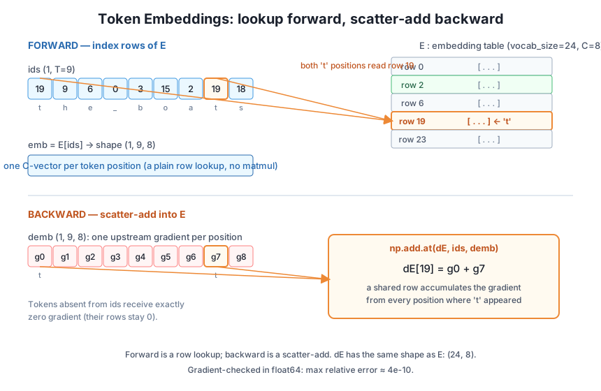
Here is the whole forward pass: to embed token id i, take row E[i]. To embed a whole batch of ids of shape (B, T), use NumPy’s fancy indexing E[ids], which returns an array of shape (B, T, C), one C-vector per position. That (B, T, C) tensor is exactly the activation shape every later module expects.

def embed_forward(E, ids):
    return E[ids]                       # (B, T) ints -> (B, T, C)

Let’s embed a short sequence. We pick the phrase "the boats" because the letter t appears twice in it, at the start and inside boats. That repetition is what makes the backward pass interesting, so keep an eye on it.

s = "the boats"
ids = np.array([encode(s)])             # (B, T) = (1, 9)
print("ids:", ids.tolist(), " ids.shape:", ids.shape)
print("token 't' id:", stoi["t"], " positions:", np.where(ids[0] == stoi["t"])[0].tolist())

emb = embed_forward(E, ids)
print("emb.shape:", emb.shape)

ids: [[19, 9, 6, 0, 3, 15, 2, 19, 18]]  ids.shape: (1, 9)
token 't' id: 19  positions: [0, 7]
emb.shape: (1, 9, 8)

The id 19 (the letter t) shows up at positions 0 and 7, and both positions look up the same row E[19]. The output is (1, 9, 8): batch of 1, nine tokens, each an 8-dimensional vector.

Why It Equals one-hot(i) @ E#

The lookup is not a trick; it is a matrix multiply in disguise. Suppose you represent token i as a one-hot vector $\mathbf{e}_i$ of length vocab_size, all zeros except a 1 in position i. Then the matrix product $\mathbf{e}_i^\top E$ selects exactly row i of E, because the single 1 picks out that row and the zeros kill every other. So

The two are identical in value. We compute it as an index instead of a matmul purely for speed: a real vocabulary has tens of thousands of rows, and multiplying a length-50000 one-hot vector (49999 of whose entries are zero) against E would waste almost all of its work. Indexing grabs the one row directly. Let’s confirm the equivalence on the first position.

onehot0 = np.zeros(vocab_size)
onehot0[ids[0, 0]] = 1.0
print("lookup == one-hot @ E at pos 0:", np.allclose(emb[0, 0], onehot0 @ E))

lookup == one-hot @ E at pos 0: True

The Backward Pass: A Scatter-Add#

Now the interesting half. During training the loss sits far downstream, and by the time gradient reaches the embedding layer we are handed demb, the gradient of the loss with respect to the embeddings, of shape (B, T, C), the same shape as emb. Our job is to turn that into dE, the gradient with respect to the table E, of shape (vocab_size, C).

Think about a single row of E, say E[19] for the letter t. In the forward pass that one row was copied to two different output positions (0 and 7). In a computational graph, when one quantity feeds several outputs, its gradient is the sum of the gradients coming back from each of those outputs, that is just the multivariate chain rule, the same rule that made dX add three projection paths in the attention backward pass. So the gradient for row 19 is the upstream gradient at position 0 plus the upstream gradient at position 7:

Read it plainly: each row of dE is the sum of the upstream gradients at every position where that token id appeared. A token that appears once contributes one term; a token that appears five times contributes five, added together; a token that never appears gets a row of zeros. This pattern, “route each incoming gradient to the row named by its id, and accumulate,” is a scatter-add.

To test it we need a scalar loss whose gradient with respect to emb we know exactly. We use the same unit-testing trick from the attention lesson: pick a fixed random tensor $G$ shaped like emb and define $L = \sum emb \cdot G$. Then dL/demb is exactly G, no chain rule needed, so we can feed a known demb into the backward pass and check what comes out.

np.random.seed(0)
G = np.random.randn(*emb.shape)         # fixed directions, (B, T, C)

def loss_from_emb(emb):
    return np.sum(emb * G)              # a scalar; dL/demb is therefore exactly G

L = loss_from_emb(emb)
demb = G                                # upstream gradient dL/demb, shape (1, 9, 8)
print("L:", round(float(L), 6))

L: -0.883398

NumPy gives us the scatter-add in one call: np.add.at(dE, ids, demb). Unlike plain fancy-indexed assignment dE[ids] += demb (which, when an id repeats, keeps only the last write and silently loses the earlier ones), np.add.at accumulates every contribution, which is precisely the summation the math demands.

def embed_backward(demb, ids, vocab_size, C):
    dE = np.zeros((vocab_size, C))      # same shape as E
    np.add.at(dE, ids, demb)           # accumulate a row for every occurrence
    return dE

dE = embed_backward(demb, ids, vocab_size, C)
print("dE.shape:", dE.shape)

dE.shape: (24, 8)

dE has the same shape as E, (24, 8), as every gradient should. Now let’s see the accumulation happen for the repeated t.

t_id = stoi["t"]                        # 19
pos = np.where(ids[0] == t_id)[0]       # [0, 7]
manual = demb[0, pos].sum(axis=0)       # sum of upstream grads at 't' positions
print("dE['t'] == sum over its", len(pos), "positions:", np.allclose(dE[t_id], manual))
print("demb at pos 0 [:3]:", np.round(demb[0, 0][:3], 6))
print("demb at pos 7 [:3]:", np.round(demb[0, 7][:3], 6))
print("dE['t']      [:3]:", np.round(dE[t_id][:3], 6))

dE['t'] == sum over its 2 positions: True
demb at pos 0 [:3]: [1.764052 0.400157 0.978738]
demb at pos 7 [:3]: [ 0.066517  0.302472 -0.634322]
dE['t']      [:3]: [1.83057  0.702629 0.344416]

Look at the first component: 1.764052 + 0.066517 = 1.830570, exactly the first entry of dE['t']. The row for t literally added together the gradients from both places it was used. This is the whole point of the scatter-add, and the reason dE[ids] += demb would be a bug: it would have recorded only the position-7 gradient and thrown away position 0.

A token that never appears in the sequence, on the other hand, was never looked up, so no gradient flows to its row and it stays zero.

absent = [i for i in range(vocab_size) if i not in ids[0]][0]
print("absent token id", absent, "row all zero:", np.allclose(dE[absent], 0.0))

absent token id 1 row all zero: True

That sparsity is a real efficiency in practice: in one training step, only the rows of the tokens actually seen in the batch get updated, no matter how large the vocabulary.

Proving It: A Numerical Gradient Check#

Shapes lining up and a hand-checked sum are encouraging, but the professional standard is a numerical gradient check: perturb one entry of E by a tiny $\epsilon$, see how much the loss moves, and compare that finite difference to our analytic dE. If the backward pass is right, they must agree for every entry. The central difference is accurate to order $\epsilon^2$:

We measure agreement with the max relative error over all entries, the largest value of $|a - n| / \max(|a|, |n|)$, where $a$ is analytic and $n$ is numerical. In float64 with $\epsilon = 10^{-5}$, a correct gradient lands around $10^{-6}$ or smaller.

def numerical_grad_E(E, ids):
    eps = 1e-5
    grad = np.zeros_like(E)
    it = np.nditer(E, flags=["multi_index"])
    while not it.finished:
        idx = it.multi_index
        orig = E[idx]
        E[idx] = orig + eps
        Lp = loss_from_emb(embed_forward(E, ids))
        E[idx] = orig - eps
        Lm = loss_from_emb(embed_forward(E, ids))
        E[idx] = orig                   # always restore the entry
        grad[idx] = (Lp - Lm) / (2 * eps)
        it.iternext()
    return grad

def max_rel_err(a, n):
    denom = np.maximum(np.abs(a), np.abs(n)) + 1e-12
    return np.max(np.abs(a - n) / denom)

num = numerical_grad_E(E, ids)
print("max relative error dE:", max_rel_err(dE, num))

max relative error dE: 4.3778003942839853e-10

A max relative error of about $4 \times 10^{-10}$, far below the $10^{-4}$ bar that separates “correct” from “buggy.” The scatter-add is exactly the gradient a brute-force perturbation of the loss produces, including for the doubled t row, whose two accumulated terms the finite difference reproduces automatically (nudging E[19] changes the loss through both of its output positions at once). Run the whole script a second time and every number is identical, because the seed fixes every random draw and the loop is deterministic; this course has no nondeterminism.

Practice Exercises#

Try these before checking the hints. They reuse E, ids, embed_forward, embed_backward, loss_from_emb, numerical_grad_E, and the tensors defined above.

Exercise 1: Break the Scatter on Purpose#

Replace the scatter-add with the buffered version dE_wrong = np.zeros_like(E); dE_wrong[ids] += demb. Compare dE_wrong[19] (the t row) against the correct dE[19], and gradient-check dE_wrong[19]. Confirm the t row is wrong while a row for a token that appears only once is still fine.

# Your code here: build dE_wrong with dE[ids] += demb, then compare
# dE_wrong[19] to dE[19] and to numerical_grad_E(E, ids)[19]

Exercise 2: Count Occurrences from dE#

Without looking at ids, you can tell how many times each token appeared from the structure of the problem. Use np.bincount(ids.ravel(), minlength=vocab_size) to count occurrences, and verify that every token with a count of zero has an all-zero row in dE, while every token with a positive count has a nonzero row.

# Your code here: counts = np.bincount(...); check zero-count rows are zero in dE

Exercise 3: Embed the Whole Corpus in Blocks#

The real training loop does not embed one phrase, it embeds batches of block_size-length windows from data. Reshape the first B * T ids of data into an (B, T) array with B = 4, T = 8, embed it, and confirm the output shape is (4, 8, 8). Then run the backward pass on a random demb of that shape and confirm dE is still (24, 8).

B, T = 4, 8
# Your code here: ids_batch = data[:B*T].reshape(B, T); embed and back-prop

Summary#

You built the first parameter block of your mini-GPT: the token embedding table that turns integer ids into learned vectors. Let’s review.

Key Concepts#

Why Embeddings

• Token ids are labels, not magnitudes, so the model must map each id to a learned vector
• The table E has shape (vocab_size, C); row i is the embedding of token i, and it is trained like any weight

Forward Pass

• Embedding token i is the lookup E[i]; a batch of ids (B, T) becomes E[ids] of shape (B, T, C)
• The lookup equals one-hot(i) @ E exactly, but indexing avoids the wasted multiply by a mostly-zero vector

Backward Pass

• The upstream gradient demb has shape (B, T, C); the table gradient dE has shape (vocab_size, C)
• Because a row is reused wherever its token appears, its gradient is the sum over those positions: dE[i] = sum of demb at every (b, t) with ids[b, t] == i
• Implement it as a scatter-add with np.add.at(dE, ids, demb), never dE[ids] += demb, which drops repeats
• Absent tokens get zero gradient; only rows for tokens seen in the batch update

Proving It

• dE has the same shape as E; a shape mismatch is a bug you catch before running
• A float64 central finite difference confirmed the scatter-add: real max relative error near $4 \times 10^{-10}$, identical on re-run

Why This Matters#

The embedding table is where a language model’s knowledge of its vocabulary lives. After training, the rows of E are not random anymore, characters and words that behave alike drift to nearby vectors, and that geometry is what every attention layer above reads and reshapes. You just built that table from nothing but an array index and a scatter-add, and proved the gradient that will train it is correct.

The scatter-add pattern is also worth carrying forward. Any time one parameter is reused across many positions, a shared embedding row, a tied output weight, a convolution kernel, its gradient accumulates over every use, and forgetting to accumulate is a bug that does not crash but quietly trains the wrong thing. You now know both the rule and the np.add.at tool that implements it safely, and you know how to prove it with a gradient check before trusting it in a real training run.

Continue Building Your Skills#

You can now turn token ids into learned vectors, but those vectors still carry no notion of where each token sits in the sequence, the embedding of t at position 0 is byte-for-byte identical to the embedding of t at position 7. That is exactly the permutation blindness this module opened with, and it is what the next lesson repairs. You will build the original transformer’s sinusoidal positional encoding, a fixed pattern of sines and cosines at geometrically spaced frequencies that stamps each position with a unique, smoothly varying signature you add straight onto the token embeddings. You will see why sinusoids of many frequencies let the model reason about relative distance, and you will generate the encoding in NumPy and add it to the (B, T, C) embeddings you produced here, taking one more step toward a complete GPT input layer.