Lesson 3 - Sinusoidal Positional Encoding

Welcome to Sinusoidal Positional Encoding#

In the last lesson you saw the problem: self-attention is permutation-equivariant. Shuffle the tokens in a sequence and the attention output shuffles the same way, because attention treats its input as a set, not an ordered list. But “the lamp keeper lights the lantern” and “the lantern lights the lamp keeper” are made of the same characters and mean very different things. Our mini-GPT has to know where each token sits.

This lesson builds the answer the original Transformer used: sinusoidal positional encoding. It is a fixed, parameter-free formula that turns a position index like 0, 1, 2, ... into a vector the same width as a token embedding, (T, C). You add that vector onto the token embeddings, and suddenly every token carries a fingerprint of its position. No weights to learn, no lookup table to store, and it keeps working at sequence lengths you never trained on.

By the end of this lesson, you will be able to:

• Write the sinusoidal encoding formula and explain what pos, i, and the 10000 constant do
• Implement sinusoidal_encoding(T, C) in pure NumPy, returning a (T, C) matrix
• Verify the three properties that make it useful: every position is unique, every value is bounded in [-1, 1], and it extrapolates to longer sequences
• Explain why relative offsets are a fixed linear rotation, and see the dot product between encodings decay as positions move apart
• Add the encoding to token embeddings without changing the (T, C) shape

You should be comfortable with NumPy slicing and the (B, T, C) shape convention from earlier modules. Let’s give our tokens a sense of place.

The Construction#

A positional encoding is a function that maps a position index pos to a C-dimensional vector, one number per embedding dimension. The Transformer paper chose to fill those dimensions with sines and cosines of different frequencies. Concretely, for position pos and dimension index i, the encoding is:

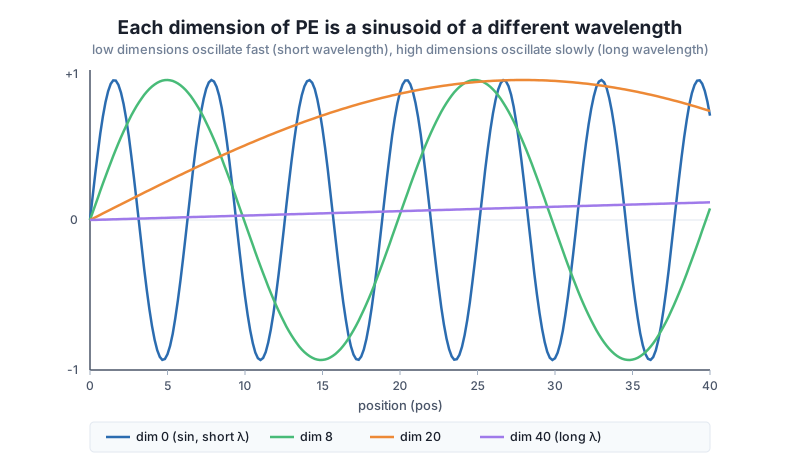
Read it slowly. Each pair of dimensions (2i, 2i+1) shares a frequency: the even one is a sine, the odd one is the matching cosine. The frequency is set by the divisor $10000^{2i/C}$. When i is small (low dimensions) the divisor is near 1, so the sinusoid completes a full cycle in just a few positions, a short wavelength. When i is large (high dimensions) the divisor grows toward 10000, so the sinusoid crawls, a long wavelength that barely moves across the whole sequence.

So the encoding of a single position is a stack of clock hands, each ticking at a different rate: fast hands in the low dimensions, slow hands in the high dimensions. Just like a combination of a seconds hand, a minutes hand, and an hours hand pins down a unique time, a combination of fast and slow sinusoids pins down a unique position.

The 10000 is just the base that sets how wide the range of wavelengths is; it lets the slowest dimension have a wavelength long enough to distinguish positions across very long sequences. It is a hyperparameter, and 10000 is the value the paper picked.

Implementing It in NumPy#

Let us turn the formula directly into code. The one subtlety is the index bookkeeping: the divisor depends on the pair index, so dimension 2i and dimension 2i+1 must use the same $10000^{2i/C}$. We handle that by computing 2 * (i // 2) for every column, which maps both members of a pair to the same exponent. Then we fill the even columns with sine and the odd columns with cosine using strided slicing.

import numpy as np
np.set_printoptions(precision=3, suppress=True)

def sinusoidal_encoding(T, C):
    # T positions (rows), C embedding dimensions (columns)
    pos = np.arange(T)[:, None]                   # (T, 1)
    i = np.arange(C)[None, :]                      # (1, C)
    div = np.power(10000.0, (2 * (i // 2)) / C)    # (1, C): same value for each dim pair
    angles = pos / div                             # (T, C): pos scaled by each frequency
    PE = np.zeros((T, C))
    PE[:, 0::2] = np.sin(angles[:, 0::2])          # even dims -> sin
    PE[:, 1::2] = np.cos(angles[:, 1::2])          # odd dims  -> cos
    return PE

T, C = 8, 16
PE = sinusoidal_encoding(T, C)
print("PE shape:", PE.shape)
print("first 3 positions, first 6 dims:")
print(PE[:3, :6])

PE shape: (8, 16)
first 3 positions, first 6 dims:
[[ 0.     1.     0.     1.     0.     1.   ]
 [ 0.841  0.54   0.311  0.95   0.1    0.995]
 [ 0.909 -0.416  0.591  0.807  0.199  0.98 ]]

There is a lot to read in those nine numbers. Look at position 0 (the top row): every sine term is $\sin(0) = 0$ and every cosine term is $\cos(0) = 1$, so position 0 encodes as an alternating 0, 1, 0, 1, .... That is always the encoding of the first token, by construction.

Now scan down a column to see the wavelengths. Column 0 (a sine in the fastest pair) climbs 0.000, 0.841, 0.909 as position goes 0, 1, 2, it is moving quickly. Column 4 (a sine in a slower pair) barely stirs: 0.000, 0.100, 0.199. That gap between a fast low dimension and a sluggish high dimension is the whole trick, and it is exactly what the figure below draws.

Property 1: Every Position Is Unique#

For an encoding to be useful, two different positions must never collapse to the same vector, otherwise the model literally cannot tell them apart. We can test this directly: compute the distance between every pair of position rows and confirm none of them is zero.

from itertools import combinations

dists = np.array([np.linalg.norm(PE[a] - PE[b]) for a, b in combinations(range(T), 2)])
print("number of position pairs:", len(dists))
print("smallest pairwise distance:", round(float(dists.min()), 4))
print("all positions unique?", bool(np.all(dists > 0)))

number of position pairs: 28
smallest pairwise distance: 1.0147
all positions unique?     True

With T = 8 there are $\binom{8}{2} = 28$ pairs of positions, and the closest two encodings are still more than 1.0 apart in Euclidean distance. No collision. Because the low dimensions oscillate quickly, even adjacent positions get visibly different codes, and because the formula is deterministic, this holds for any T you choose.

Property 2: Every Value Is Bounded#

The encoding is made only of sines and cosines, so every entry lives in [-1, 1] no matter how large pos gets. This matters because you are about to add the encoding onto the token embeddings; if positional values could blow up with position, late tokens in a long sequence would be dominated by their position and lose their identity.

print("min value:", round(float(PE.min()), 4))
print("max value:", round(float(PE.max()), 4))
print("in [-1, 1]?", bool(np.all(PE >= -1.0) and np.all(PE <= 1.0)))

min value: -0.99
max value: 1.0
in [-1, 1]? True

Bounded and well behaved. A learned embedding table could in principle drift to huge values; the sinusoidal formula is guaranteed to stay in range for position 5 or position 5 million.

Property 3: Relative Position Is a Linear Function#

Here is the property that makes attention love this encoding. Because each dimension pair is a (sin, cos) at a fixed frequency, shifting a position by a constant offset $k$ is the same as applying a fixed rotation to that pair, one that depends on $k$ but not on the absolute position. In matrix form, $PE_{pos+k} = R_k \, PE_{pos}$ for a rotation $R_k$ that is the same everywhere along the sequence.

That means a linear layer inside attention can, in principle, learn to detect “the token 3 positions back” as a single fixed transform, rather than memorizing a separate rule for every absolute position. We can see a downstream consequence of this structure numerically: the dot product between two encodings depends mostly on how far apart the positions are, and it tends to decay as the gap grows. Let us measure the dot product of position 3 against every other position.

ref = 3
print("PE[3] . PE[j]:")
for j in range(T):
    print(f"  j={j}  offset |3-j|={abs(ref-j)}  dot={float(PE[ref] @ PE[j]):.3f}")

PE[3] . PE[j]:
  j=0  offset |3-j|=3  dot=5.543
  j=1  offset |3-j|=2  dot=6.368
  j=2  offset |3-j|=1  dot=7.485
  j=3  offset |3-j|=0  dot=8.000
  j=4  offset |3-j|=1  dot=7.485
  j=5  offset |3-j|=2  dot=6.368
  j=6  offset |3-j|=3  dot=5.543
  j=7  offset |3-j|=4  dot=5.560

Read the dot column. A position’s encoding is most similar to itself (dot = 8.000, which is close to $C/2 = 8$ since each of the 8 cosine-pair contributions peaks at 1), and the similarity falls off almost symmetrically as you move away in either direction: 7.485 at offset 1, 6.368 at offset 2, 5.543 at offset 3. The value is a smooth, near-symmetric function of the offset alone, not of the absolute indices, which is the fingerprint of that fixed-rotation structure. Averaging over every starting position sharpens the same trend:

print("average PE[i] . PE[i+offset]:")
for off in range(4):
    vals = [float(PE[i] @ PE[i+off]) for i in range(T-off)]
    print(f"  offset {off}: {np.mean(vals):.3f}")

average PE[i] . PE[i+offset]:
  offset 0: 8.000
  offset 1: 7.485
  offset 2: 6.368
  offset 3: 5.543

A clean monotone decay: 8.000 -> 7.485 -> 6.368 -> 5.543 as the offset grows. Attention, which scores tokens with exactly this kind of dot product, can pick up on that signal to prefer nearby positions.

Property 4: It Extrapolates#

Because the encoding is a formula, not a learned lookup table, it is defined for every position, including positions longer than anything you trained on. A learned table of size (max_len, C) simply has no row for position max_len + 1; the sinusoidal function just evaluates $\sin$ and $\cos$ at a larger argument and returns a valid, in-range, unique vector.

short = sinusoidal_encoding(8, 16)     # a sequence we might train on
long = sinusoidal_encoding(100, 16)    # much longer than training

# The first 8 rows of the long encoding are identical to the short one
print("shared prefix matches?", np.allclose(short, long[:8]))
print("row 99 exists and is in range:",
      bool(np.all(long[99] >= -1) and np.all(long[99] <= 1)))

shared prefix matches? True
row 99 exists and is in range: True

Position 3 always encodes the same way whether the sequence is 8 or 100 long, and position 99 is perfectly well defined even if training only ever saw 8 tokens. That consistency is why a model with sinusoidal encoding can be run on longer inputs than it was trained on without the position machinery breaking.

Adding It to Token Embeddings#

Finally, how does the mini-GPT use this? The rule is simple: add the positional encoding to the token embeddings, element for element. Both are (T, C), so the sum is (T, C), and each token vector now carries a component that says “I am at position t.” There are no positional parameters to train; the encoding is fixed and just gets added in every forward pass.

rng = np.random.default_rng(42)
tok_emb = rng.normal(0, 1, size=(T, C)) * 0.1   # stand-in for a real token embedding lookup
PE = sinusoidal_encoding(T, C)

X = tok_emb + PE                                  # inject position

print("token emb:", tok_emb.shape, "+ PE:", PE.shape, "-> X:", X.shape)
print("X[0, :4]:", X[0, :4])

token emb: (8, 16) + PE: (8, 16) -> X: (8, 16)
X[0, :4]: [0.03  0.896 0.075 1.094]

The shape is unchanged: (T, C) goes in, (T, C) comes out, so the rest of the network (attention, the feed-forward block) does not need to know positional encoding exists. It just receives token vectors that happen to encode order. In the real mini-GPT this addition is the very first thing that happens after the token embedding lookup, and everything downstream builds on it.

Practice Exercises#

Try these before checking the hints. They reuse sinusoidal_encoding from above.

Exercise 1: Confirm Position 0 Is Always [0, 1, 0, 1, ...]#

Generate an encoding for C = 8 and check that row 0 is exactly the alternating pattern of zeros and ones, for any T you pick.

# Your code here: build PE and inspect PE[0]

Exercise 2: Watch a Column’s Wavelength Grow#

For T = 40 and C = 16, print how far the sine value in column 0 moves between positions 0 and 1, and compare it to column 14. Explain which oscillates faster and why.

# Your code here: compare PE[1, 0] - PE[0, 0] against PE[1, 14] - PE[0, 14]

Exercise 3: Show the Dot Product Is Offset-Symmetric#

Pick position 4 in an encoding with T = 9, and confirm that PE[4] . PE[4 - k] is approximately equal to PE[4] . PE[4 + k] for k = 1, 2, 3. What does that symmetry tell you about the encoding?

# Your code here: compare dot products at equal offsets on each side of position 4

Summary#

You gave the mini-GPT a sense of order without adding a single trainable parameter. Sinusoidal positional encoding turns a position index into a (T, C) vector that you add straight onto the token embeddings, and it does so with a formula that is unique, bounded, relative-position-friendly, and defined at any length.

Key Concepts#

The Construction

• $PE_{pos, 2i} = \sin(pos / 10000^{2i/C})$ and $PE_{pos, 2i+1} = \cos(pos / 10000^{2i/C})$
• Each dimension pair is a (sin, cos) at a fixed frequency; low dimensions have short wavelengths, high dimensions have long ones
• The 10000 base sets how wide the range of wavelengths spans

The Four Properties

• Unique: every position gets a distinct vector (all 28 pairwise distances were > 1.0 for T = 8)
• Bounded: every value stays in [-1, 1], so position never overwhelms content
• Relative: an offset $k$ is a fixed rotation $R_k$; the dot product decayed 8.000 -> 7.485 -> 6.368 -> 5.543 with offset
• Extrapolates: it is a formula, so position 99 is defined even after training only on length 8

Usage

• X = tok_emb + PE, both (T, C), so the shape is preserved and no parameters are added
• The addition happens once, right after token embedding lookup, before attention

Why This Matters#

Self-attention has no built-in notion of order, and yet order is the whole point of language. Sinusoidal positional encoding was the original, elegant fix: a closed-form function that injects position for free and, thanks to its (sin, cos) pairing, hands attention a clean linear handle on relative distance. Every early Transformer, and the machine-translation model that started it all, ran on exactly this encoding.

It also frames a design question you will meet everywhere: should position be a fixed formula or a learned parameter? The sinusoidal approach costs nothing to store and extrapolates gracefully, but it bakes in a fixed structure the model cannot adjust. The next lesson takes the opposite bet.

Continue Building Your Skills#

You now have a parameter-free way to tell your mini-GPT where each token sits, and you have seen the three guarantees, uniqueness, bounded values, and graceful extrapolation, that make the sinusoidal formula more than a clever trick. Hold on to the picture of stacked clock hands ticking at different rates, because it explains at a glance why far-apart positions still get distinguishable codes. In the next lesson we swap the fixed formula for learned positional embeddings: instead of computing position with sines and cosines, we give the model a trainable table of position vectors, one row per slot, and let gradient descent decide what “position 5” should mean. You will build that lookup table, compare its trade-offs against the sinusoidal encoding you just wrote, and see why modern GPT-style models, including the one you are building, often reach for the learned version.