Lesson 4 - Learned Positional Embeddings

Welcome to Learned Positional Embeddings#

In the previous lesson you built sinusoidal positional encoding: a fixed formula of sines and cosines that stamps each position with a unique pattern, no training required. It is elegant, but it is not what GPT actually does. This lesson teaches the approach the real GPT-2 uses instead, and it is almost embarrassingly simple: a learned positional embedding, a plain lookup table of position vectors that the model trains like any other weight.

Our mini-GPT already has a token embedding that maps each character id to a vector. Here you add its twin: a positional table P where row t holds the embedding for position t. To tell the model where each token sits in the sequence, you add these two embeddings together. That sum, token_emb + P[:T], is the input the rest of the transformer will attend over in later modules.

By the end of this lesson, you will be able to:

• Define a learned positional embedding table P of shape (block_size, C) and explain what each row means
• Add P[:T] to a batch of token embeddings with the correct broadcast
• Contrast learned positional embeddings with sinusoidal ones: flexibility versus extrapolation, parameters versus none
• Derive the backward pass for P as a batch-summed slice-add and implement it in NumPy
• Verify the positional-embedding gradient with a float64 numerical gradient check
• Explain why a learned table cannot represent any position beyond block_size

You should be comfortable with NumPy broadcasting, the (B, T, C) activation shape from earlier modules, and the numerical gradient check pattern from the backpropagation lessons. Let’s build the table.

A Table of Positions#

A learned positional embedding is nothing more than a matrix of parameters. If your context length is block_size and your model width is C (the n_embd from our config), then

is a table with one row per position. Row P[0] is the vector the model uses to mean “I am at position 0,” P[1] means “position 1,” and so on up to P[block_size - 1]. These numbers start out random and are updated by gradient descent exactly like the weights in an attention head or an MLP. The model gets to decide, on its own, what each position should feel like.

This is the whole difference from Lesson 3. Sinusoidal encoding computes the position vector from a formula; a learned embedding stores it in a table and lets training fill it in. There is no clever math inside P, just parameters.

For a sequence of length T (which must satisfy $T \le \text{block\_size}$), you only need the first T rows. Positions in the sequence are always the dense integers 0, 1, 2, ..., T-1, so the slice P[:T] gives you exactly the position vectors you need, in order.

The Forward Pass: Add P[:T]#

Token embeddings for a batch flow as (B, T, C): B sequences, each T tokens long, each token a C-vector. The positional slice P[:T] has shape (T, C), the same for every sequence in the batch, because position 3 means the same thing in sequence 0 as it does in sequence 1. So the forward pass is a single broadcast add:

In NumPy that is literally token_emb + P[:T]. The (T, C) array broadcasts across the leading batch axis of the (B, T, C) token embeddings, adding the same position vector to every sequence at that position.

Let’s build it for real. We use a tiny config, block_size = 8 and C = 4, so the shapes are easy to read, with a small init scale of * 0.02 (real transformers init positional tables near this scale). Everything is seeded so the run is reproducible.

import numpy as np

np.random.seed(42)

block_size = 8   # max positions the table supports
C = 4            # model width (n_embd), tiny for readability
B, T = 2, 5      # batch, sequence length (T <= block_size)

# Learned positional embedding table: row t is the embedding for position t
P = np.random.randn(block_size, C).astype(np.float64) * 0.02

# Token embeddings for a batch of sequences (B, T, C)
token_emb = np.random.randn(B, T, C).astype(np.float64)

# Forward: add the position slice P[:T] to every sequence in the batch
out = token_emb + P[:T]                      # broadcast (B,T,C) + (T,C)

print("P shape:        ", P.shape)
print("token_emb shape:", token_emb.shape)
print("out shape:      ", out.shape)

P shape:         (8, 4)
token_emb shape: (2, 5, 4)
out shape:       (2, 5, 4)

The output keeps the token embedding shape (2, 5, 4), exactly what we want: adding position information does not change the shape, it only shifts each token vector by its position’s vector. Notice that P has 8 rows but we only touched the first 5 (P[:5]); the last three rows sit unused for a length-5 sequence, a detail that matters both for the backward pass and for the block_size limit below.

The Backward Pass: A Batch-Summed Slice-Add#

Since the forward pass is just an addition, its backward pass is beautifully simple. Suppose the rest of the network hands us an upstream gradient dout of shape (B, T, C) (the gradient of the loss with respect to out). Addition passes gradient straight through, so the gradient with respect to the token embeddings is simply

The interesting part is dP. The subtlety is that a single row P[t] was added into every sequence in the batch at position t. When one value feeds multiple outputs, its gradient is the sum of the gradients from all of them. So the gradient for position t accumulates across the whole batch:

That sum is over the batch axis, giving a (T, C) result that we scatter back into the first T rows of a full (block_size, C) gradient. Rows T through block_size - 1 were never used, so their gradient is exactly zero. Because the used positions are the dense integers 0..T-1, this “scatter” is really just a slice assignment, far simpler than the token-embedding backward pass (Lesson 5), where the used rows are scattered token ids that can repeat.

# Upstream gradient from the rest of the network
rng = np.random.default_rng(0)
dout = rng.standard_normal((B, T, C))

# out = token_emb + P[:T], broadcast over batch.
# dtoken_emb = dout (addition passes gradient straight through)
# dP[:T] = sum of dout over the batch axis; rows T..block_size-1 stay zero.
dtoken_emb = dout
dP = np.zeros_like(P)
dP[:T] = dout.sum(axis=0)                     # slice-add into dense rows 0..T-1

print("dP shape:       ", dP.shape)
print("dP rows T..end (unused positions) all zero?:", np.allclose(dP[T:], 0.0))

dP shape:        (8, 4)
dP rows T..end (unused positions) all zero?: True

dP has the same shape as P, (8, 4), which is the reassuring rule that a gradient always matches the shape of the thing it belongs to. And the unused rows 5 through 7 are all zero, confirming that positions the sequence never reached receive no gradient. Each used row is the sum of that position’s gradient across the two sequences in the batch.

Proving It: A Float64 Gradient Check#

Shapes lining up is encouraging, but it does not prove the numbers are right. As in every backward-pass lesson, we settle it with a numerical gradient check in float64: nudge each entry of P by a tiny $\epsilon$, measure how the loss changes, and compare that finite difference to our analytic dP.

To make dout play the role of a real upstream gradient, we use a linear surrogate loss $L = \sum (\text{out} \odot \text{dout})$. Its derivative with respect to out is exactly dout, so the analytic dP we computed above should match the finite-difference estimate to high precision.

def loss_fn(P_):
    o = token_emb + P_[:T]
    return np.sum(o * dout)                   # surrogate loss with dL/dout = dout

eps = 1e-6
dP_num = np.zeros_like(P)
for i in range(P.shape[0]):
    for j in range(P.shape[1]):
        Pp = P.copy(); Pp[i, j] += eps
        Pm = P.copy(); Pm[i, j] -= eps
        dP_num[i, j] = (loss_fn(Pp) - loss_fn(Pm)) / (2 * eps)

num = np.abs(dP - dP_num)
den = np.maximum(1e-12, np.abs(dP) + np.abs(dP_num))
max_rel_err = np.max(num / den)
print(f"dP max relative error: {max_rel_err:.3e}")

dP max relative error: 2.876e-08

A max relative error around $3 \times 10^{-8}$, far below the 1e-6 bar, means the analytic and numerical gradients agree to nearly machine precision in float64. The slice-add backward pass is correct. Note the check naturally covers the unused rows too: for positions 5 through 7 both the analytic gradient and the finite difference are zero (perturbing P[6] does not change a length-5 output at all), and they agree trivially.

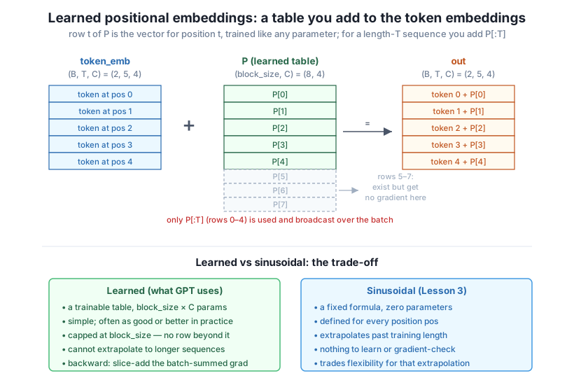
The block_size Limit#

The learned table buys simplicity at one real cost: it only knows the positions it was given rows for. P has exactly block_size rows, so it can represent positions 0 through block_size - 1 and no more. Ask for position block_size and there is simply no row to return, NumPy raises an IndexError.

print("block_size =", block_size, "-> valid positions are 0 ..", block_size - 1)
try:
    _ = P[block_size]        # a position the table never learned
except IndexError as e:
    print("Indexing position", block_size, "raises IndexError:", e)

block_size = 8 -> valid positions are 0 .. 7
Indexing position 8 raises IndexError: index 8 is out of bounds for axis 0 with size 8

This is exactly why GPT-2 has a hard context window: the model literally has no embedding for a position past its trained block_size. Sinusoidal encoding does not share this limit, its formula produces a valid vector for any integer position, so it can (in principle) extrapolate to sequences longer than anything seen in training.

So which should you use? In practice, learned positional embeddings usually match or beat sinusoidal ones on the sequence lengths they were trained on, and they cost only block_size * C extra parameters, which is tiny next to the rest of a transformer. GPT-2 chose them for exactly that reason. The trade-off is flexibility (the model tunes each position freely) versus extrapolation (sinusoidal generalizes to unseen lengths, learned cannot). For our fixed-context mini-GPT, where every sequence is at most block_size long, the learned table is both simpler and the historically faithful choice.

Practice Exercises#

Try these before checking the hints. They reuse P, token_emb, dout, block_size, B, T, and C from the code above.

Exercise 1: A Single-Sequence Sanity Check#

With a batch of B = 1, the batch sum in the backward pass has only one term, so dP[:T] should equal dout[0] exactly. Build a (1, T, C) upstream gradient, compute dP with the same slice-add rule, and confirm dP[:T] matches dout[0] with np.allclose.

# Your code here: make dout1 of shape (1, T, C), compute dP, compare dP[:T] to dout1[0]

Exercise 2: Confirm the Unused Rows Get No Gradient#

Pick an unused position like t = 6 (valid because 6 < block_size but 6 >= T). Perturb P[6, 0] by $\pm \epsilon$, recompute the surrogate loss with loss_fn, and show numerically that its gradient is zero, matching dP[6, 0].

# Your code here: finite-difference dP[6, 0] using loss_fn and compare to dP[6, 0]

Exercise 3: Feel the Extrapolation Gap#

Write a one-line guard that would let sinusoidal encoding handle a position of block_size + 3 but must reject it for the learned table. Explain in a comment why the learned table cannot serve that position.

# Your code here: attempt to fetch position block_size + 3 from P, and describe
# what a sinusoidal formula would do instead

Summary#

You built the positional approach GPT actually ships with: a learned table you add to token embeddings and train by gradient descent. Let’s review.

Key Concepts#

The Learned Table

• A learned positional embedding is a trainable matrix P of shape (block_size, C); row t is the embedding for position t
• Unlike sinusoidal encoding, there is no formula inside P, the values are parameters that training fills in
• GPT-2 uses this approach

Forward Pass

• For a length-T sequence, add the slice P[:T] (shape (T, C)) to the token embeddings (B, T, C)
• The add broadcasts across the batch: out = token_emb + P[:T], since position t means the same thing in every sequence
• The output keeps the (B, T, C) shape, position info shifts each vector without reshaping

Backward Pass

• dtoken_emb = dout (addition passes gradient straight through)
• dP[:T] = dout.sum(axis=0) — sum over the batch, because each position row was added once per sequence
• Rows T..block_size-1 stay zero; the used rows are dense 0..T-1, so it is a slice-add, not a scattered scatter
• Verified with a float64 numerical gradient check: max relative error $\approx 2.9 \times 10^{-8}$

The Trade-off

• Learned: simple, often as good or better in practice, but capped at block_size and cannot extrapolate; costs block_size * C parameters
• Sinusoidal: a formula with zero parameters that extrapolates to any position
• Indexing past block_size raises IndexError, the model has no embedding for positions it never trained

Why This Matters#

Every GPT you have used inherits the two facts from this lesson. First, the model’s fixed context window, the reason a chat assistant “forgets” text past a certain length, is a direct consequence of the learned table having exactly block_size rows and no more. Second, the reason adding a positional embedding works at all is the same reason you will meet again and again in transformers: attention is permutation-invariant, so order has to be injected as data, and a learned vector per position is the most direct way to do it.

The backward pass you derived, a gradient that sums across every place a parameter was reused, is the same pattern that governs the token embedding you build next and, more broadly, every shared parameter in a network. Once you see “used in k places, so its gradient is the sum of k terms,” the backward pass of embeddings, weight tying, and even convolution stops being mysterious.

Continue Building Your Skills#

You now have both halves of a transformer’s input, the token embedding from earlier and the positional embedding from this lesson, sitting in the same C-dimensional space, ready to be summed. In the next lesson you will assemble them into a single embedding layer: a small, reusable component that takes a batch of token ids, looks up their token vectors, adds P[:T], and returns the (B, T, C) input the rest of the mini-GPT will attend over. You will implement its forward pass, then its full backward pass, and this is where the trickier scatter of the token-embedding gradient (repeated ids accumulating into the same row) finally shows up, a direct sequel to the clean slice-add you just proved correct here.