Lesson 1 - Q, K, V: The Three Projections

Welcome to Q, K, V: The Three Projections#

In Module 1 you turned a fixed content-based lookup into a learnable one by projecting the input through three weight matrices. That was the moment attention became trainable. This module takes that idea apart bolt by bolt until you have a complete, gradient-checked self-attention layer, and it starts here, by giving those three projections their precise definitions.

The word that matters in this module is self. In self-attention, the query, the key, and the value all come from the same input sequence: a sequence looks at itself. That single design choice is what lets each position in your mini-GPT gather context from every other position in the same block of text. In this lesson you formalize the three projections $W_q, W_k, W_v$ that make it work, pin down every shape, count the parameters training will learn, and then prove something that surprises many people the first time they see it: self-attention is not symmetric. The fact that position $i$ attends strongly to position $j$ tells you nothing about how much $j$ attends to $i$, and you will see exactly why in NumPy.

By the end of this lesson, you will be able to:

• Explain what makes attention self-attention, and contrast it with cross-attention
• Describe the distinct role and geometry of each projection: $W_q$, $W_k$, and $W_v$
• Track the shapes through a head: X is (B, T, C), the weights are (C, hs), and Q, K, V are (B, T, hs)
• Count the learnable parameters in one head as $3 \cdot C \cdot hs$
• Show in NumPy that because $W_q \neq W_k$, Q differs from K and the score matrix $QK^\top$ is not symmetric

You should be comfortable with the projected attention head from Module 1 Lesson 4 and with NumPy matrix multiplication and broadcasting. There is no training here, only the forward projections and their shapes. Let’s begin.

What Makes It Self-Attention#

Attention, in general, answers a question of the form: given a set of queries and a set of key/value pairs, what mix of values should each query read? Nothing in that description says the queries and the keys have to come from the same place. What makes an attention layer self-attention is precisely that they do: every query, key, and value is computed from one input sequence $X$. The sequence is both the thing asking questions and the thing being asked about.

Concretely, given an input $X$ of shape $(B, T, C)$, a stack of $T$ token vectors each of width $C$, self-attention forms all three ingredients from that same $X$:

Every one of the $T$ positions produces a query (what it is looking for), a key (what it offers to others), and a value (what it contributes if selected). Position 3 can then look at position 7’s key, and if they match, read position 7’s value, all within the same sequence. This is how your mini-GPT will let the token at the end of a phrase pull in information from tokens earlier in the same block.

The alternative is cross-attention, where the queries come from one sequence and the keys and values come from a different one. A translation decoder, for example, forms queries from the sentence it is generating but keys and values from the encoded source sentence, so each output word can look back at the input. The math is identical; only the source of $X$ differs. Your GPT is a decoder-only model, so it uses self-attention throughout, but it is worth knowing that the same three-projection machinery covers both cases.

Three Roles, Three Matrices#

Why three separate matrices instead of one? Because a token plays three genuinely different roles in an attention step, and forcing one vector to serve all three would tie the model’s hands. Give each role its own learned projection and the three can specialize independently.

The query, $W_q$: “what am I looking for?” Multiplying a token’s vector by $W_q$ maps it into a query space whose geometry encodes the kind of information this position wants to retrieve. A token that represents a verb might learn to produce a query that points toward subjects; a token at a phrase boundary might query for the phrase’s start. The query is the search request.

The key, $W_k$: “what do I offer to be found by?” The matrix $W_k$ maps each token into a key space. A key is the advertisement a position posts so that other positions’ queries can find it. Crucially the key space is a different learned space from the query space, so “what this token is looking for” and “what this token is worth matching against” need not coincide.

The value, $W_v$: “what do I contribute if chosen?” Once the query/key match decides how much each position is attended to, $W_v$ decides what actually flows through. It maps each token into a value space, the content that gets mixed into the output. Separating value from key means a token can be highly findable on one kind of cue while contributing content of an entirely different character.

Because $W_q$, $W_k$, and $W_v$ are independent parameter matrices, the query space, key space, and value space can all differ in geometry. This separation is the whole reason attention is expressive rather than a fixed similarity rule, and it is exactly what training will shape.

The Shapes, Precisely#

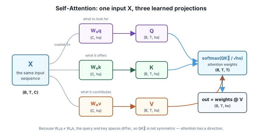
Getting the shapes right is most of the battle, so let’s nail them down before touching code. Recall the course conventions: batch size $B$, sequence length $T$ (at most block_size), model width $C$ (this is n_embd), and head size $hs$.

• The input activations flow as $X$: $(B, T, C)$.
• Each projection matrix $W_q, W_k, W_v$: $(C, hs)$. It maps a $C$-dimensional token to an $hs$-dimensional one.
• The multiply $X W_q$ contracts the last axis of $X$ (size $C$) against the first axis of $W_q$ (size $C$), leaving $Q$: $(B, T, hs)$. Same for $K$ and $V$.

Notice that the head size $hs$ does not have to equal the model width $C$. In a single-head toy you might set them equal, but real transformers use multi-head attention: they split the width across several heads, so each head works in a smaller subspace of size $hs = C / n\_head$. In our mini-GPT config, $C = 64$ and $n\_head = 4$, so each head has $hs = 16$. The projections deliberately step down from $C = 64$ to $hs = 16$; Module 3 stitches four such heads back together. For now, just remember: $W$ is $(C, hs)$, and $hs$ is a design choice, not forced to match $C$.

The parameter count follows immediately. One head has three matrices, each with $C \cdot hs$ entries, so it learns

weights (biases are usually omitted in attention projections, and we omit them). For our real head that is $3 \cdot 64 \cdot 16 = 3072$ numbers. These matrices are the only thing an attention head learns; everything else, the dot product, the scaling, the softmax, has no parameters at all. When people say a transformer “learns what to attend to,” they mean gradient descent is tuning exactly these $W_q, W_k, W_v$ entries.

Building the Projections in NumPy#

Time to make this concrete on our running example. We take a short slice of the Lantern Bay corpus, embed each character into a $C$-dimensional vector to form $X$, then project it. We use a small demo width $C = 8$ and head size $hs = 4$ so every array is small enough to read, and we seed everything with 42 for reproducibility.

import numpy as np

CORPUS = (
    "the lamp keeper walks the shore at dusk. "
    "the lamp keeper lights the lantern when the fog rolls in. "
    "the boats come home when the lantern glows. "
    "the boats wait outside the bay when the fog is thick. "
    "a small boat drifts near the rocks at dawn. "
    "the keeper rings the bell when a boat drifts near the rocks. "
    "the tide rises at dusk and falls at dawn. "
    "the gulls call over the bay when the tide is low. "
    "the keeper counts the boats and writes the count in a book. "
    "the lantern burns all night and rests at dawn. "
) * 20

chars = sorted(set(CORPUS))
vocab_size = len(chars)
stoi = {c: i for i, c in enumerate(chars)}
encode = lambda s: [stoi[c] for c in s]

np.random.seed(42)
C = 8                              # model width for this demo (mini-GPT uses 64)
embed_table = np.random.randn(vocab_size, C)

text = "the lamp"
ids = encode(text)
X = embed_table[ids][None, :, :]   # (B, T, C)
B, T, _ = X.shape

print("vocab_size:", vocab_size)
print("slice:", repr(text), "ids:", ids)
print("X shape:", X.shape, "(B, T, C)")
# Output:
# vocab_size: 24
# slice: 'the lamp' ids: [19, 9, 6, 0, 12, 2, 13, 16]
# X shape: (1, 8, 8) (B, T, C)

We have one sequence ($B = 1$) of $T = 8$ characters, each embedded into a $C = 8$ vector. Now create the three projection matrices and apply them. We scale the random init by * 0.1: real transformers init these near * 0.02, but that small a scale makes the eventual attention weights nearly uniform and hard to inspect, so for demos in this module we use a slightly larger scale so the numbers differentiate visibly. The * 0.1 choice does not affect any of the shape or symmetry facts below; it only makes the printed values easier to read.

hs = 4                             # head size, deliberately smaller than C
Wq = np.random.randn(C, hs) * 0.1
Wk = np.random.randn(C, hs) * 0.1
Wv = np.random.randn(C, hs) * 0.1

Q = X @ Wq                         # (B, T, hs)
K = X @ Wk                         # (B, T, hs)
V = X @ Wv                         # (B, T, hs)

print("Wq/Wk/Wv shape:", Wq.shape, "(C, hs)")
print("Q shape:", Q.shape, "(B, T, hs)")
print("K shape:", K.shape)
print("V shape:", V.shape)
print("learned params in one head:", 3 * C * hs, "= 3 * C * hs")
print("real mini-GPT head (C=64, hs=16):", 3 * 64 * 16, "params")
# Output:
# Wq/Wk/Wv shape: (8, 4) (C, hs)
# Q shape: (1, 8, 4) (B, T, hs)
# K shape: (1, 8, 4)
# V shape: (1, 8, 4)
# learned params in one head: 96 = 3 * C * hs
# real mini-GPT head (C=64, hs=16): 3072 params

Every shape matches the table above: three (8, 4) matrices turn an (1, 8, 8) input into three (1, 8, 4) tensors. The head steps the width down from $C = 8$ to $hs = 4$, and it holds $3 \cdot 8 \cdot 4 = 96$ learnable numbers. Scaling up to the real config, one head carries 3072 parameters, and those are the only weights an attention head owns.

Why Self-Attention Is Not Symmetric#

Here is the payoff of using three separate matrices, and a fact that trips up almost everyone the first time. Because $W_q$ and $W_k$ are different matrices, the query a token produces is generally not equal to the key it produces. Let’s look at the first token, 't':

np.set_printoptions(precision=4, suppress=True)
print("Q[0,0]:", Q[0, 0])
print("K[0,0]:", K[0, 0])
print("Q[0,0] equals K[0,0]?", np.allclose(Q[0, 0], K[0, 0]))
# Output:
# Q[0,0]: [0.4591 0.827  0.179  0.0736]
# K[0,0]: [-0.1142 -0.1084  0.2109  0.0254]
# Q[0,0] equals K[0,0]? False

Same token, same input vector, but its query and its key are entirely different vectors, because they went through different learned maps. This is the essential asymmetry of self-attention. When the model computes how much position $i$ attends to position $j$, it takes the dot product of position $i$’s query with position $j$’s key:

Swap $i$ and $j$ and you get $Q_j \cdot K_i$, a completely different quantity, because $Q_j \neq K_j$ and $Q_i \neq K_i$. So the score matrix $QK^\top$ is not symmetric. (The $\frac{1}{\sqrt{hs}}$ scaling is Lesson 2’s subject; we include it here so the pipeline is complete, but it does not affect symmetry.)

scores = Q @ K.transpose(0, 2, 1) / np.sqrt(hs)   # (B, T, T)
print("scores shape:", scores.shape, "(B, T, T)")
print("scores[0, 0, 1]:", round(float(scores[0, 0, 1]), 4), " (query 0 -> key 1)")
print("scores[0, 1, 0]:", round(float(scores[0, 1, 0]), 4), " (query 1 -> key 0)")
print("scores[0] symmetric?", np.allclose(scores[0], scores[0].T))
# Output:
# scores shape: (1, 8, 8) (B, T, T)
# scores[0, 0, 1]: -0.1481  (query 0 -> key 1)
# scores[0, 1, 0]: -0.0016  (query 1 -> key 0)
# scores[0] symmetric? False

Position 0 attending to position 1 scores $-0.1481$, while position 1 attending to position 0 scores $-0.0016$. Different numbers, from the same pair of tokens, just in opposite directions. That is exactly what we want: how much the article 't'… wants to look at the space after it is a separate question from how much that space wants to look back. Had we reused one matrix for both query and key ($W_q = W_k$), the scores would be forced symmetric and the model could never express a one-way relationship.

Completing the Forward Pass#

The projections and scores are the new material; the rest of the head is the scaled dot-product attention you met in Module 1. Turn the scores into weights with a numerically stable softmax over the last axis, then read a weighted mixture of the values. The point of running it here is to confirm the whole head executes end to end and that each output position’s attention is a valid probability distribution.

def softmax(x, axis=-1):
    x = x - x.max(axis=axis, keepdims=True)   # subtract row max for stability
    e = np.exp(x)
    return e / e.sum(axis=axis, keepdims=True)

weights = softmax(scores, axis=-1)   # (B, T, T)
out = weights @ V                    # (B, T, hs)

print("weights shape:", weights.shape, "| out shape:", out.shape)
print("weights[0] row sums:", weights[0].sum(axis=-1))
print("every row sums to 1?", np.allclose(weights.sum(axis=-1), 1.0))
# Output:
# weights shape: (1, 8, 8) | out shape: (1, 8, 4)
# weights[0] row sums: [1. 1. 1. 1. 1. 1. 1. 1.]
# every row sums to 1? True

Each of the eight rows of weights sums to 1: row $t$ is the distribution over which positions token $t$ reads from. Multiplying by $V$ mixes the value vectors according to those distributions, producing an output of shape (B, T, hs), one $hs$-dimensional context vector per position. Run the whole script a second time and every printed number is identical, because the seed fixes the embedding table and all three projection matrices. That determinism is exactly what lets you trust the shape and symmetry checks above.

You have now built a complete single-head self-attention forward pass from three learned matrices, and you have proven the property that separates real attention from a naive symmetric similarity: it has a direction.

Practice Exercises#

Try these before checking the hints. They reuse X, Wq, Wk, Wv, and the variables defined above.

Exercise 1: Force Symmetry by Sharing a Matrix#

Set the key projection equal to the query projection (Wk_shared = Wq), recompute K, the scores, and check whether the score matrix is now symmetric. Explain in a comment why sharing the matrix produces a symmetric result.

# Your code here: build K with Wq, recompute scores, test symmetry

Exercise 2: Change the Head Size#

Rebuild Wq, Wk, Wv with hs = 6 instead of 4 (keep C = 8), recompute Q, K, V, and print their shapes and the new parameter count. Confirm the score matrix shape does not change even though the head size did.

# Your code here: set hs = 6, remake the three matrices, reproject, print shapes

Exercise 3: Confirm V Uses Its Own Space#

Print V[0, 0] and compare it to Q[0, 0] and K[0, 0] from the lesson. Then set Wv = Wk and recompute V; describe what now equals what, and argue in a comment why giving the value its own matrix matters for expressiveness.

# Your code here: inspect V[0,0], then try Wv = Wk and recompute V

Summary#

You gave self-attention’s three projections their precise definitions and proved the asymmetry that makes attention directional. Let’s review.

Key Concepts#

Self-Attention

• In self-attention, $Q$, $K$, and $V$ are all projections of the same input $X$: a sequence attends to itself
• Cross-attention is identical math with $Q$ from one sequence and $K$, $V$ from another; a decoder-only GPT uses self-attention throughout

Three Roles, Three Matrices

• $W_q$ maps each token to a query (what it is looking for), $W_k$ to a key (what it offers to be matched against), $W_v$ to a value (what content it contributes)
• The three are separate learned matrices, so the query, key, and value spaces can each have a different geometry

Shapes and Parameters

• $X$ is (B, T, C); each of $W_q, W_k, W_v$ is (C, hs); $Q, K, V$ are each (B, T, hs)
• Head size $hs$ need not equal model width $C$; multi-head attention uses $hs = C / n\_head$ (our config: $64 / 4 = 16$)
• One head learns $3 \cdot C \cdot hs$ weights (3072 for the real head), the only parameters an attention head has

Why Attention Is Directional

• Because $W_q \neq W_k$, a token’s query differs from its key, so Q[0,0] differs from K[0,0]
• Therefore $QK^\top$ is not symmetric: scores[0,0,1] (-0.1481) differs from scores[0,1,0] (-0.0016)
• Sharing $W_q = W_k$ would force symmetry and destroy the ability to express one-way relationships
• Softmax over the last axis makes every row a distribution (each sums to 1) before mixing the values

Why This Matters#

Every transformer you will ever use, from a tiny character model to a frontier language model, is built out of the three projections you just formalized. When a model “learns what to attend to,” gradient descent is tuning exactly these $W_q, W_k, W_v$ matrices and nothing else in the attention step. Understanding that the query, key, and value are three different learned views of the same input, and that their separateness is what makes attention directional and expressive, is the mental model that makes everything downstream, multi-head attention, masking, and the backward pass, click into place.

It also inoculates you against a common misconception. Attention is not a symmetric similarity like a correlation matrix; it is a directed, learned lookup. The token that gathers information and the token that provides it play different roles, encoded by different matrices, and that asymmetry is a feature language genuinely needs. Hold on to the picture of one $X$ fanning out into three spaces, because the next several lessons all operate inside that picture.

Continue Building Your Skills#

You now have $Q$, $K$, and $V$ as three separate projections of one input, and you have seen that their dot products form an asymmetric score matrix. The obvious next question is the one we quietly deferred: why did we divide those scores by $\sqrt{hs}$? In the next lesson you will build scaled dot-product attention in full and run a real experiment that shows the $1/\sqrt{hs}$ factor is not cosmetic. Without it, dot products grow with the head size, the softmax saturates into a near one-hot spike, and the gradients that training relies on collapse toward zero. You will watch that failure happen in NumPy, then watch the scaling fix it, and in doing so understand why every transformer divides by the square root of the head dimension.