Lesson 2 - Scaled Dot-Product Attention

Welcome to Scaled Dot-Product Attention#

In the previous lesson you gave attention its three learned projections: an input $X$ becomes a query $Q$, a key $K$, and a value $V$. You already know the rest of the recipe informally, compare queries to keys, softmax the scores, average the values. This lesson writes that recipe as the single formula every transformer runs, examines each piece, and then focuses hard on one small factor buried inside it: the division by $\sqrt{d_k}$. That factor looks like a cosmetic detail. It is not. Without it, a self-attention layer stops learning as soon as the head grows wide, and you will prove exactly why with a real NumPy experiment rather than taking anyone’s word for it.

This is the operation at the heart of the mini-GPT you are building. Every attention head in every block will call the scaled_dot_product_attention function you write here, so it is worth getting the formula, and the reasoning behind the scale, completely solid.

By the end of this lesson, you will be able to:

• Write the canonical attention formula $\text{softmax}(QK^\top/\sqrt{d_k})\,V$ and name the shape of every intermediate
• Explain why a dot product of two random vectors has variance that grows with their dimension $d_k$
• Prove, with a real experiment, that raw score variance tracks $d_k$ while dividing by $\sqrt{d_k}$ pins it near 1
• Show that an unscaled softmax at large $d_k$ collapses into a near one-hot spike that kills gradients
• Implement the reusable scaled_dot_product_attention(Q, K, V) forward and confirm its shapes and row sums

You should be comfortable with the query/key/value projections from Lesson 1 and with NumPy matrix multiplication and broadcasting. A little probability, the idea that variances of independent terms add, helps for the proof, and we rebuild it as we go. Let’s begin.

The Full Formula, Piece by Piece#

Here is the operation, written the way you will see it in every paper and codebase:

It looks dense, but it is just four steps chained together, and you have met all four before. Take them left to right, keeping the shapes in view. Work with a single head on a batch of sequences: $Q$, $K$, and $V$ are each of shape (B, T, d_k), where B is the batch size, T is the sequence length, and $d_k$ is the head size (the brief calls it hs; the attention literature calls it $d_k$, the dimension of the keys, and we use that name here to match the formula).

Step 1: $Q K^\top$, all pairwise scores. For every query position you want a raw similarity against every key position, and the dot product measures that. Multiplying $Q$ of shape (B, T, d_k) by $K^\top$ of shape (B, d_k, T) gives a (B, T, T) matrix. Entry $(i, j)$ is the dot product of query $i$ with key $j$, a single number saying how much position $i$ is drawn to position $j$. This is the full table of every position against every position.

Step 2: divide by $\sqrt{d_k}$. Each of those dot products is a sum of $d_k$ products, so as the head gets wider the raw scores get larger, purely because there are more terms to add. Dividing by $\sqrt{d_k}$ rescales them back to a stable size. This is the whole subject of the lesson, and the next sections prove it is necessary. The shape does not change; it is still (B, T, T).

Step 3: softmax over the last axis. Each row of the (B, T, T) score matrix is turned into a probability distribution over the T key positions, using the numerically stable softmax (subtract the row max, exponentiate, normalize). After this, every row is non-negative and sums to 1: these are the attention weights, still (B, T, T).

Step 4: multiply by $V$. Finally, weight the value vectors. Multiplying the (B, T, T) weights by $V$ of shape (B, T, d_k) gives a (B, T, d_k) output. Row $i$ of the result is the weighted average of all value vectors, using position $i$’s attention distribution as the weights. Each token leaves with a blend of content pulled from wherever it chose to look.

That is the entire mechanism: score, scale, normalize, average. Three of the four steps you already implemented in Module 1. The one piece we have not justified is the scale, so we turn to it now.

Why a Dot Product Grows With Dimension#

The scores in step 1 are dot products. To understand why they need rescaling, look at what a dot product actually is when the vectors are random.

Suppose the entries of $Q$ and $K$ are independent, with mean 0 and variance 1, which is roughly true early in training when weights are freshly initialized. A single score is the dot product of one query vector $q$ and one key vector $k$, each of length $d_k$:

Each term $q_i k_i$ is a product of two independent zero-mean unit-variance numbers. Its expected value is 0, and its variance is 1 (the variance of a product of independent mean-zero unit-variance variables is the product of their variances, $1 \times 1 = 1$). Now sum $d_k$ of these independent terms. Variances of independent quantities add, so the variance of the whole sum is:

The score has variance $d_k$. Its typical magnitude, the standard deviation, is therefore $\sqrt{d_k}$. Double the head size and the scores spread out by $\sqrt{2}$; go from $d_k = 16$ to $d_k = 256$ and the typical score magnitude grows by a factor of four. This is not a property of any particular data; it is pure arithmetic of adding up more terms.

The fix falls right out of the algebra. If a random variable has variance $d_k$, dividing it by $\sqrt{d_k}$ divides its variance by $d_k$, bringing it back to 1:

So dividing by $\sqrt{d_k}$ keeps the score variance at roughly 1 no matter how wide the head is. That is precisely the $\sqrt{d_k}$ in the formula, and it is the reason the scores stay comparable across head sizes. Now let us watch it happen for real.

Proving It: Score Variance Tracks d_k#

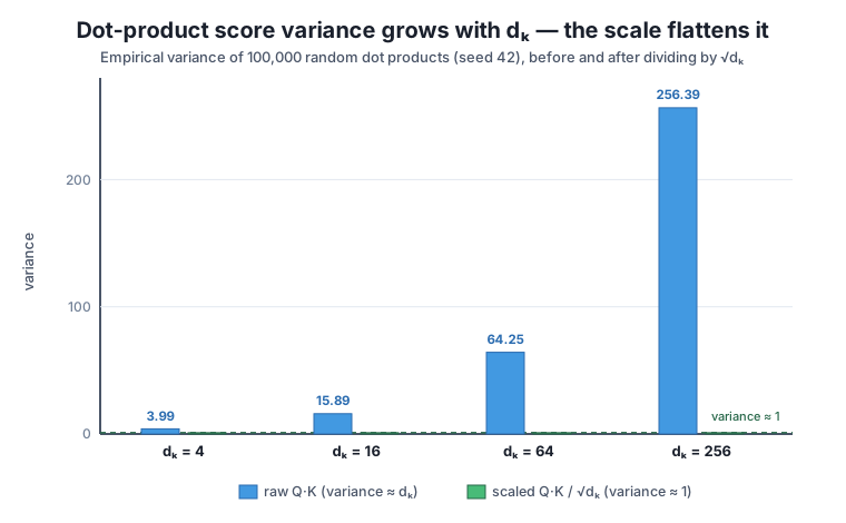
Enough algebra, let us measure it. The plan: for several values of $d_k$, draw a hundred thousand random query and key vectors, compute one dot-product score per pair, and print the empirical variance. The theory says the raw variance should track $d_k$ (about 4, 16, 64, 256) and the scaled variance should sit near 1 in every case.

import numpy as np

np.random.seed(42)
n_samples = 100_000
print("d_k | var(raw scores) | var(scores / sqrt(d_k))")
for d_k in [4, 16, 64, 256]:
    Q = np.random.randn(n_samples, d_k)     # zero-mean, unit-variance
    K = np.random.randn(n_samples, d_k)
    scores = np.sum(Q * K, axis=1)          # one dot product per sample
    raw_var = scores.var()
    scaled_var = (scores / np.sqrt(d_k)).var()
    print(f"{d_k:>3} | {raw_var:>15.3f} | {scaled_var:>.4f}")

d_k | var(raw scores) | var(scores / sqrt(d_k))
  4 |           3.988 | 0.9971
 16 |          15.891 | 0.9932
 64 |          64.249 | 1.0039
256 |         256.391 | 1.0015

Read the middle column: the raw variance is 3.99, 15.89, 64.25, 256.39, which is essentially $d_k$ itself at every row, exactly as the algebra predicted. The scores really do grow with dimension. Now read the right column: after dividing by $\sqrt{d_k}$, the variance is 0.9971, 0.9932, 1.0039, 1.0015, flat at 1 regardless of whether the head has 4 dimensions or 256. One small division cancels the entire dimensional growth. This is not a coincidence of the seed; it is the $\frac{d_k}{d_k} = 1$ identity from the previous section showing up in real numbers.

Why Large Scores Break Softmax#

Growing variance would be harmless if softmax did not care about the absolute size of its inputs. But it cares enormously. Softmax exponentiates its inputs, so a gap of a few units between the largest score and the rest becomes an astronomical ratio after exp. When the scores have standard deviation $\sqrt{d_k}$, the biggest score at $d_k = 256$ sits many units above its neighbors, and softmax turns that gap into a near one-hot spike, almost all the weight on a single position.

Let us see it. Take one query and eight competing keys at $d_k = 256$, and compare the softmax of the raw scores against the softmax of the scaled scores. We measure two things: the largest weight (how peaked the distribution is) and its entropy (how spread out it is; higher entropy means more spread, with $\log 8 \approx 2.079$ being perfectly uniform).

import numpy as np

def softmax(x, axis=-1):
    x = x - x.max(axis=axis, keepdims=True)   # subtract row max for stability
    e = np.exp(x)
    return e / e.sum(axis=axis, keepdims=True)

np.random.seed(42)
d_k = 256
T = 8                                    # eight competing key positions
q = np.random.randn(d_k)
Kmat = np.random.randn(T, d_k)
raw_scores = Kmat @ q                     # (8,) one query vs 8 keys
scaled_scores = raw_scores / np.sqrt(d_k)

w_unscaled = softmax(raw_scores)
w_scaled = softmax(scaled_scores)
entropy = lambda p: float(-np.sum(p * np.log(p + 1e-12)))

print("raw_scores      :", np.round(raw_scores, 2))
print("scaled_scores   :", np.round(scaled_scores, 2))
print("unscaled softmax:", np.round(w_unscaled, 4))
print("scaled softmax  :", np.round(w_scaled, 4))
print(f"unscaled max weight = {w_unscaled.max():.4f}  entropy = {entropy(w_unscaled):.4f}")
print(f"scaled   max weight = {w_scaled.max():.4f}  entropy = {entropy(w_scaled):.4f}")
print(f"uniform entropy (log {T}) = {np.log(T):.4f}")

raw_scores      : [ -3.12  13.41 -27.    12.41   2.39  24.29  -1.23  -2.77]
scaled_scores   : [-0.2   0.84 -1.69  0.78  0.15  1.52 -0.08 -0.17]
unscaled softmax: [0. 0. 0. 0. 0. 1. 0. 0.]
scaled softmax  : [0.0634 0.1781 0.0142 0.1673 0.0894 0.3514 0.0713 0.0648]
unscaled max weight = 1.0000  entropy = 0.0003
scaled   max weight = 0.3514  entropy = 1.7909
uniform entropy (log 8) = 2.0794

Look at the raw scores: they range from $-27$ to $+24$, a spread of about fifty, exactly the $\sqrt{256} = 16$-scale magnitude the theory predicted. Softmax turns that spread into [0, 0, 0, 0, 0, 1, 0, 0], all the weight on position 5 and essentially nothing anywhere else. The max weight is 1.0000 and the entropy is 0.0003, a near-perfect one-hot spike. The scaled scores, the same numbers divided by 16, range from $-1.69$ to $+1.52$. Their softmax is [0.063, 0.178, 0.014, 0.167, 0.089, 0.351, 0.071, 0.065], still leaning toward position 5 (weight 0.35) but keeping real weight on the others. Its entropy is 1.79, close to the uniform maximum of 2.08. Same query, same keys, one factor of $\sqrt{d_k}$ between a distribution that looks at everything and one that has collapsed onto a single position.

Why does the one-hot spike matter? Because of the gradient. The derivative of softmax is proportional to $p_i(1 - p_i)$ and cross-terms $-p_i p_j$. When one $p$ is 1 and the rest are 0, every one of those terms is 0: the softmax is saturated and passes essentially no gradient backward. A layer stuck in that state cannot learn, because attention receives no signal about how to adjust its scores. The scale is what keeps softmax in its responsive, high-gradient regime as the model grows wide. This connects straight back to the vanishing-gradient trouble you saw with saturated sigmoids in the deep-learning foundations: a saturated nonlinearity is a dead end for learning, and an unscaled attention score walks right into one.

The Canonical Forward in NumPy#

You now have every reason the formula is written the way it is. Here it is as one reusable function, the non-causal scaled dot-product attention that every head in your mini-GPT will call. It takes $Q$, $K$, $V$ already projected (Lesson 1’s job) and returns both the output and the attention weights, so later lessons can inspect what the head attended to.

import numpy as np

def softmax(x, axis=-1):
    x = x - x.max(axis=axis, keepdims=True)   # subtract row max for stability
    e = np.exp(x)
    return e / e.sum(axis=axis, keepdims=True)

def scaled_dot_product_attention(Q, K, V):
    # Q, K, V: (B, T, d_k)
    d_k = Q.shape[-1]
    scores = Q @ K.transpose(0, 2, 1) / np.sqrt(d_k)   # (B, T, T)
    weights = softmax(scores, axis=-1)                 # (B, T, T)
    out = weights @ V                                  # (B, T, d_k)
    return out, weights

Feed it a small random batch and print the shape at every stage. We use a fixed seed so the run is fully reproducible.

rng = np.random.default_rng(42)
B, T, d_k = 1, 6, 16
Q = rng.standard_normal((B, T, d_k))
K = rng.standard_normal((B, T, d_k))
V = rng.standard_normal((B, T, d_k))

out, weights = scaled_dot_product_attention(Q, K, V)
print("Q/K/V:", Q.shape, " scores/weights:", weights.shape, " out:", out.shape)
print("weights row sums:", np.round(weights.sum(-1), 6))
print("weights[0]:")
print(np.round(weights[0], 3))

Q/K/V: (1, 6, 16)  scores/weights: (1, 6, 6)  out: (1, 6, 16)
weights row sums: [[1. 1. 1. 1. 1. 1.]]
weights[0]:
[[0.057 0.41  0.13  0.21  0.104 0.09 ]
 [0.072 0.606 0.025 0.089 0.079 0.128]
 [0.172 0.162 0.096 0.093 0.185 0.291]
 [0.116 0.108 0.216 0.123 0.173 0.263]
 [0.056 0.104 0.27  0.301 0.05  0.219]
 [0.1   0.083 0.496 0.134 0.107 0.081]]

Match that against the formula. $Q$, $K$, $V$ came in at (1, 6, 16); the $QK^\top$ comparison produced a (1, 6, 6) score table; softmax over the last axis normalized every row (each sums to 1.0, confirmed); and the weighted average of the values left at (1, 6, 16). Because the scores were scaled, the weights are differentiated but not collapsed, position 1 leans on key 1 (weight 0.606) and position 5 on key 2 (0.496), while every row keeps meaningful weight elsewhere. That healthy spread is exactly what the $\sqrt{d_k}$ division bought you, and it is what will let gradients flow when this head is trained in Module 7.

Practice Exercises#

Try these before checking the hints. They reuse the softmax and scaled_dot_product_attention functions and the experiments above.

Exercise 1: Measure the Variance at d_k = 1024#

The lesson tested $d_k$ up to 256. Extend the sweep to $d_k = 1024$: draw random $Q$ and $K$, compute the raw dot-product variance and the scaled variance, and confirm the raw variance is near 1024 while the scaled variance stays near 1.

# Your code here (reuse np.random.seed(42) and the Experiment 1 pattern)

Exercise 2: Sweep the Softmax Entropy Across d_k#

Show the collapse happening gradually. For $d_k$ in [4, 16, 64, 256], build one query against eight keys, take the softmax of the unscaled raw scores, and print its entropy. Watch the entropy fall toward 0 as $d_k$ grows.

# Your code here: loop over d_k, build q and Kmat, softmax(Kmat @ q), print entropy

Exercise 3: Confirm Scaling Does Not Change the Ranking#

The scale changes the sharpness of the attention distribution but not the order of the scores. For one query against eight keys at d_k = 256, confirm that the unscaled and scaled softmax weights produce the same argsort (the same ranking of positions), even though the actual weights differ wildly.

# Your code here: compare argsort of w_unscaled and w_scaled

Summary#

You assembled the complete scaled dot-product attention formula and proved, with real numbers, why the $\sqrt{d_k}$ scale is not optional. Let’s review.

Key Concepts#

The Formula

• $\text{Attention}(Q, K, V) = \text{softmax}\!\left(\frac{QK^\top}{\sqrt{d_k}}\right) V$, four steps: score, scale, normalize, average
• Shapes: $Q, K, V$ are (B, T, d_k); $QK^\top$ and the weights are (B, T, T); the output is (B, T, d_k)
• Softmax runs over the last axis, so every row of the weights is a probability distribution over key positions

Why the Scale Exists

• A dot product of two zero-mean unit-variance vectors of length $d_k$ has variance $d_k$, because $d_k$ independent unit-variance terms add up
• Its typical magnitude is therefore $\sqrt{d_k}$; dividing by $\sqrt{d_k}$ returns the variance to 1 at any head size
• The experiment confirmed it: raw variance 3.99, 15.89, 64.25, 256.39 for $d_k$ = 4, 16, 64, 256; scaled variance 0.9971, 0.9932, 1.0039, 1.0015

Why It Matters for Learning

• Large scores push softmax into a near one-hot spike: at $d_k = 256$ the unscaled max weight was 1.0000 with entropy 0.0003
• A saturated softmax passes almost no gradient, so the head cannot learn; the scaled version kept entropy at 1.79 (of a possible 2.08)
• Divide by $\sqrt{d_k}$, not $d_k$ — the standard deviation grows like $\sqrt{d_k}$, and that is what you rescale by

The Implementation

• scaled_dot_product_attention(Q, K, V) returns the (B, T, d_k) output and the (B, T, T) weights
• Verified shapes flow (1, 6, 16) → (1, 6, 6) → (1, 6, 16), and every attention row summed to 1

Why This Matters#

Scaled dot-product attention is the single operation that defines the transformer. Everything else in the architecture, multiple heads, stacked blocks, causal masking, positional information, is scaffolding around this one formula. The $\sqrt{d_k}$ factor is easy to dismiss as a magic constant when you read it in a paper, but you have now derived it from the variance of a sum and watched an unscaled softmax collapse into a dead, gradient-free spike. That is the difference between copying a formula and owning it.

The lesson also handed you a durable debugging instinct. When a wide attention layer refuses to learn, or its weights look suspiciously one-hot, you will know to check the scale and to read the entropy of the distribution before suspecting anything more exotic. And when you meet the same $\sqrt{d_k}$ inside a multi-head attention block later in the course, you will not have to relearn why it is there. It keeps the scores comparable, softmax responsive, and gradients alive, no matter how wide the model grows.

Continue Building Your Skills#

You can now compute the full attention output and, just as important, the attention weights themselves. So far you have only glanced at those weights to confirm they sum to 1. In the next lesson you will slow down and learn to read the attention matrix as a diagnostic instrument: each row as a per-position distribution over what a token looked at, the argmax as its strongest link, the entropy as a measure of how focused or diffuse its attention is. You will run the head over a real slice of the Lantern Bay corpus and interpret which characters lean on which, turning the (B, T, T) table from a shape you verify into a picture you can actually understand, the last piece of intuition before Module 2 derives the backward pass through everything you have built.