Lesson 3 - The Attention Matrix: Who Attends to Whom

Welcome to The Attention Matrix#

In the previous lesson you built scaled dot-product attention and saw why dividing the scores by $\sqrt{hs}$ keeps the softmax from saturating. Your self_attention function already returns two things: the output vectors and a weights array of shape (B, T, T). So far you have mostly cared about the output. This lesson turns the spotlight on that second return value, the attention matrix, because it is the most interpretable object in the entire transformer. Read it well and you can see, position by position, exactly where your tiny char-level GPT is looking.

The attention matrix is where the abstract phrase “the sequence attends to itself” becomes a concrete grid of numbers you can print and inspect. Every row is a decision: for this one position, how should I spread my attention across all the positions in the context? Learning to read that grid is a skill you will use for the rest of the course, whether you are debugging a head that has collapsed onto a single token or admiring one that has learned to track structure.

By the end of this lesson, you will be able to:

• Interpret each row of the (T, T) attention matrix as a probability distribution over key positions, and confirm the rows sum to 1
• Distinguish the diagonal (self-attention) from the off-diagonal (cross-position mixing), and tell a focused row from a diffuse one
• Explain why the attention matrix is generally not symmetric, and verify it with max|A - A.T| > 0
• Show that without positional information, identical characters produce identical rows, and connect that gap to the positional encoding you will add in Module 4

You should be comfortable with the self_attention function from Lesson 2, softmax as a row-wise normalizer, and the Lantern Bay corpus and char-level tokenizer from Module 1. Let’s begin.

What the (T, T) Matrix Really Is#

When self-attention runs on a sequence of length $T$, it produces a square matrix of weights, call it $A$, of shape (T, T). This matrix is the answer to a single question asked $T$ times over: for each position, how much does it draw from every position, including itself?

Formally, entry $A_{ij}$ is the weight that query position $i$ places on key position $j$. It comes straight out of the softmax you already wrote:

The softmax is taken over the last axis, meaning it normalizes across $j$ for each fixed $i$. That single design choice fixes how you must read the matrix:

• Read it row by row. Row $i$ is a complete probability distribution: $T$ non-negative numbers that sum to 1. It tells you how position $i$ blends the other positions when it builds its output vector.
• A column is not a distribution. Column $j$ collects how much every position attends to $j$. Those numbers need not sum to anything in particular.

The output for position $i$ is just that row used as mixing weights over the value vectors: $\text{out}_i = \sum_j A_{ij}\, v_j$. So a row that is peaked on one column copies almost one value vector; a row spread evenly averages many. The matrix is the mixing plan.

Setting Up a Real Slice to Inspect#

Talking about the matrix is one thing; printing a real one is better. We will take a short, real slice of the Lantern Bay corpus, tokenize it with the same char-level scheme from Module 1, embed it, and run one attention head. Everything is seeded so you get the exact numbers shown here.

First the corpus and tokenizer, verbatim from Module 1:

import numpy as np
np.set_printoptions(precision=2, suppress=True)

CORPUS = (
    "the lamp keeper walks the shore at dusk. "
    "the lamp keeper lights the lantern when the fog rolls in. "
    "the boats come home when the lantern glows. "
    "the boats wait outside the bay when the fog is thick. "
    "a small boat drifts near the rocks at dawn. "
    "the keeper rings the bell when a boat drifts near the rocks. "
    "the tide rises at dusk and falls at dawn. "
    "the gulls call over the bay when the tide is low. "
    "the keeper counts the boats and writes the count in a book. "
    "the lantern burns all night and rests at dawn. "
) * 20

chars = sorted(set(CORPUS))
vocab_size = len(chars)
stoi = {c: i for i, c in enumerate(chars)}
itos = {i: c for i, c in enumerate(chars)}
encode = lambda s: [stoi[c] for c in s]
decode = lambda ids: "".join(itos[i] for i in ids)

print("vocab_size:", vocab_size)

vocab_size: 24

Now pick a 10-character slice. We deliberately choose "the lamp k" because it contains the space character twice (at positions 3 and 8). That repetition will let us demonstrate something important later, so it is worth choosing on purpose.

text = "the lamp k"
ids  = encode(text)
T    = len(text)
print("slice:", repr(text))
print("ids:  ", ids)
print("T:    ", T)

slice: 'the lamp k'
ids:   [19, 9, 6, 0, 12, 2, 13, 16, 0, 11]
T:     10

Notice the token id 0 appears at index 3 and index 8: those are the two spaces, and they encode to the same integer. Hold that thought.

Embedding and Running One Head#

We now embed each character and run a single attention head. Two deliberate choices about scale matter here.

First, the embedding. Each character id looks up a row of an embedding table. For this inspection we use a unit-scale random table (randn, no shrinking) so different characters get genuinely different vectors and the attention has something to distinguish.

Second, the projection scale. As the brief for this course stresses, real transformers initialize Wq, Wk, Wv around * 0.02, but at that scale the query-key dot products are tiny, the softmax comes out nearly uniform, and every row of the matrix looks like a flat 0.10, 0.10, ... with nothing to read. To inspect structure we use a larger demo init of * 0.5. This does not change the mechanism at all; it just makes the differences between positions visible on the page.

np.random.seed(42)
C  = 16          # embedding width
hs = 16          # head size (single head, hs = C here)

embed_table = np.random.randn(vocab_size, C)   # unit-scale (demo init)
X = embed_table[ids][None, :, :]               # (B=1, T=10, C=16)

Wq = np.random.randn(C, hs) * 0.5              # demo init * 0.5 so structure shows
Wk = np.random.randn(C, hs) * 0.5
Wv = np.random.randn(C, hs) * 0.5

print("X shape:", X.shape)

X shape: (1, 10, 16)

Here is the same scaled dot-product attention you built in Lesson 2, returning both the output and the weight matrix:

def softmax(x, axis=-1):
    x = x - x.max(axis=axis, keepdims=True)
    e = np.exp(x)
    return e / e.sum(axis=axis, keepdims=True)

def self_attention(X, Wq, Wk, Wv):
    Q, K, V = X @ Wq, X @ Wk, X @ Wv           # each (B, T, hs)
    hs = Q.shape[-1]
    scores = Q @ K.transpose(0, 2, 1) / np.sqrt(hs)   # (B, T, T)
    weights = softmax(scores, axis=-1)          # (B, T, T)
    return weights @ V, weights

out, weights = self_attention(X, Wq, Wk, Wv)
A = weights[0]                                  # (T, T) for our single sequence
print("out shape:", out.shape)
print("A shape:  ", A.shape)

out shape: (1, 10, 16)
A shape:   (10, 10)

The output is (1, 10, 16), one 16-dimensional vector per position. But the object we came for is A, the (10, 10) matrix of weights. Let’s look at it.

Reading the Matrix#

print("Attention matrix A (rows = query i, cols = key j):")
print(np.round(A, 2))

Attention matrix A (rows = query i, cols = key j):
[[0.08 0.1  0.02 0.01 0.06 0.09 0.   0.64 0.01 0.  ]
 [0.03 0.01 0.   0.39 0.02 0.02 0.   0.05 0.39 0.09]
 [0.   0.   0.03 0.42 0.02 0.   0.07 0.   0.42 0.03]
 [0.   0.36 0.01 0.   0.   0.   0.   0.62 0.   0.  ]
 [0.01 0.78 0.08 0.   0.   0.   0.1  0.01 0.   0.  ]
 [0.   0.   0.   0.   0.97 0.03 0.   0.   0.   0.  ]
 [0.   0.02 0.   0.   0.   0.   0.97 0.   0.   0.  ]
 [0.   0.   0.   0.   0.   0.   1.   0.   0.   0.  ]
 [0.   0.36 0.01 0.   0.   0.   0.   0.62 0.   0.  ]
 [0.   0.   0.03 0.19 0.01 0.   0.13 0.46 0.19 0.  ]]

Ten rows, ten columns, and the characters of "the lamp k" label both axes: index 0 is t, 1 is h, 2 is e, 3 is a space, 4 is l, and so on. Let’s translate a few rows from numbers into words.

• Row 7 (the p) is maximally focused. It reads [0, 0, 0, 0, 0, 0, 1, 0, 0, 0]. All of its weight, 1.00, lands on column 6 (the m). Position 7 builds its output almost entirely from position 6’s value vector. This is a peaked row: attention has committed to a single source.
• Row 1 (the h) is diffuse. It reads [0.03, 0.01, 0, 0.39, 0.02, 0.02, 0, 0.05, 0.39, 0.09]. No single column dominates; the mass is split, most notably 0.39 on column 3 and 0.39 on column 8. This is a flat, averaging row: position 1’s output is a blend of several positions rather than a copy of one.
• Row 0 (the t) leans on one neighbor but hedges. Its largest weight is 0.64 on column 7 (the p), with small crumbs scattered elsewhere. It is more focused than row 1 but less absolute than row 7.

That vocabulary, peaked versus flat, focused versus diffuse, is how practitioners describe attention heads at a glance. A head whose rows are all peaked is doing hard selection; a head whose rows are all flat is doing soft averaging. Both are useful, and a trained model ends up with a mix.

Before reading further, confirm the one property every row must satisfy:

print("row sums:     ", np.round(A.sum(axis=1), 6))
print("rows sum to 1?", np.allclose(A.sum(axis=1), 1.0))

row sums:      [1. 1. 1. 1. 1. 1. 1. 1. 1. 1.]
rows sum to 1? True

Every row sums to exactly 1, which is the softmax doing its job across the key axis. If a row of an attention matrix ever fails this check, the softmax axis is wrong.

The Diagonal Is Self-Attention#

The grid has a special line running through it: the diagonal, the entries $A_{ii}$ where the query position and the key position are the same. Each diagonal entry answers “how much does position $i$ attend to itself?” Everything off the diagonal is cross-position mixing: pulling information from other positions.

print("diagonal (self-attention):", np.round(np.diag(A), 2))

diagonal (self-attention): [0.08 0.01 0.03 0.   0.   0.03 0.97 0.   0.62 0.  ]

In this untrained, demo-scaled head the diagonal is mostly small: position 1 keeps only 0.01 for itself and hands the rest to its neighbors, while position 6 (the m) keeps 0.97, attending almost entirely to itself. There is no rule that a position must attend to itself; whether the diagonal is large depends entirely on how the query and key of each position align. In trained models the diagonal often carries meaningful weight, because a token’s own content is frequently the most useful thing it has, but it is a learned outcome, never a built-in.

The distinction is worth naming because you will use it constantly when reading heads. A strong diagonal means positions are largely preserving their own content; a weak diagonal with strong off-diagonal bands means the sequence is actively shuffling information between positions. Attention is exactly this mixture of “keep myself” and “gather from others,” laid out as a grid.

Why the Matrix Is Not Symmetric#

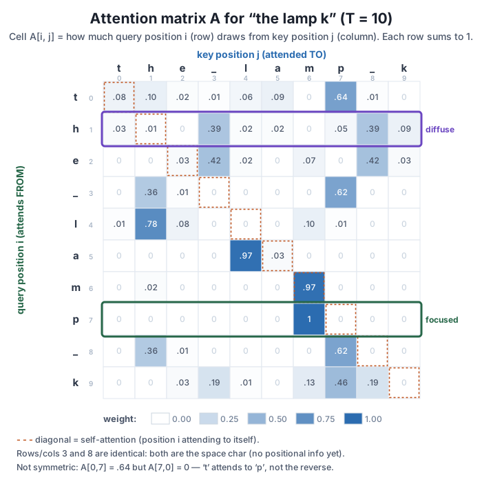
A natural assumption, and a common early mistake, is that attention is mutual: if position $i$ attends strongly to $j$, surely $j$ attends strongly back to $i$. The matrix says otherwise. Attention is a directed relationship, and $A$ is generally not symmetric: $A_{ij} \neq A_{ji}$.

The reason is baked into the mechanism. The score for $(i, j)$ uses position $i$’s query against position $j$’s key: $q_i \cdot k_j$. The score for $(j, i)$ uses position $j$’s query against position $i$’s key: $q_j \cdot k_i$. Because the query and key projections are different learned matrices ($W_q \neq W_k$), swapping $i$ and $j$ swaps a query for a key on both sides, and there is no reason the two dot products should match. Query and key play asymmetric roles: one asks, the other answers.

We can see it directly in our matrix. Compare position 0 asking about position 7 with position 7 asking about position 0:

print("A[0, 7] (t -> p):", round(float(A[0, 7]), 2))
print("A[7, 0] (p -> t):", round(float(A[7, 0]), 2))

asym = np.max(np.abs(A - A.T))
print("max|A - A.T|:", round(float(asym), 4))
print("symmetric?  ", np.allclose(A, A.T))

A[0, 7] (t -> p): 0.64
A[7, 0] (p -> t): 0.0
max|A - A.T|: 0.9963
symmetric?   False

Position 0 (the t) pours 0.64 of its attention into position 7 (the p), but position 7 sends nothing back to position 0. The largest disagreement anywhere in the matrix, max|A - A.T|, is 0.9963, essentially a full unit of weight. This is not a bug or a quirk of our seed; it is the fundamental nature of dot-product attention. A - A.T is the matrix of these disagreements, and its largest absolute entry being well above zero is the crisp numerical statement of “attention is a one-way street.”

Identical Characters, Identical Rows#

Now the payoff for choosing a slice with two spaces. Positions 3 and 8 are both the space character, so they encode to the same id (0) and therefore look up the same embedding vector. Nothing else in a single attention head depends on where a token sits, only on its content vector. So what happens to their rows?

print("chars:", list(text))
print("A[3]:", np.round(A[3], 2))
print("A[8]:", np.round(A[8], 2))
print("row 3 == row 8?      ", np.allclose(A[3], A[8]))
print("max|row3 - row8|:    ", round(float(np.max(np.abs(A[3] - A[8]))), 8))

chars: ['t', 'h', 'e', ' ', 'l', 'a', 'm', 'p', ' ', 'k']
A[3]: [0.   0.36 0.01 0.   0.   0.   0.   0.62 0.   0.  ]
A[8]: [0.   0.36 0.01 0.   0.   0.   0.   0.62 0.   0.  ]
row 3 == row 8?       True
max|row3 - row8|:     0.0

The two rows are exactly identical, down to the last bit. The space at position 3 and the space at position 8 produce the same query vector, so they compute the same scores against every key, so the softmax hands them the same distribution. The model literally cannot tell the two spaces apart. This is the same limitation you first met in Module 1 Lesson 5: self-attention on its own is permutation-blind. It sees a bag of content vectors, not an ordered sequence. Shuffle the positions and, apart from relabeling, the same rows come out.

That is a real problem for language, where order carries meaning: “the boat drifts” and “drifts the boat” are not the same. The fix is not to change attention, which is elegant precisely because it is order-agnostic, but to inject order into the inputs before attention runs. In Module 4 you will add positional encoding: a position-dependent signal blended into each embedding so that the space at position 3 and the space at position 8 arrive with different vectors, and their rows are free to differ. For now, seeing two identical rows is the clean, concrete evidence that the position information simply is not there yet.

Practice Exercises#

Try these before checking the hints. They reuse A, X, Wq, Wk, Wv, text, and the self_attention function from above.

Exercise 1: Find Each Position’s Top Source#

For every query position $i$, find the key position it attends to most and how much weight it places there. Print each as position i (char) -> position j (char): weight. This turns the grid into a plain-language summary of who looks at whom.

# Your code here: use np.argmax along axis 1 of A

Exercise 2: Quantify How Focused Each Row Is#

A peaked row and a flat row differ in how concentrated their weight is. Compute the largest weight in each row (A.max(axis=1)) as a simple focus score, and identify the most focused and the most diffuse query positions. Confirm your answer matches the highlighted rows in the figure.

# Your code here: max weight per row tells you focus

Exercise 3: Break the Identical-Rows Tie with a Position Signal#

Rows 3 and 8 are identical because the two spaces share an embedding. Add a tiny position-dependent nudge to the embeddings before attention, X_pos = X + 0.3 * np.arange(T).reshape(1, T, 1), rerun attention, and check whether rows 3 and 8 are still equal. Explain in a comment what changed and why this previews positional encoding.

# Your code here: build X_pos, rerun self_attention, compare rows 3 and 8

Summary#

You learned to read the single most interpretable object in a transformer: the attention matrix. It is no longer a mysterious weights array but a grid you can print, translate into words, and sanity-check.

Key Concepts#

The (T, T) Matrix

• Entry $A_{ij}$ is the weight query position $i$ places on key position $j$; it comes from a softmax over the key axis
• Read it row by row: each row is a probability distribution over positions that sums to 1
• A column is incoming attention and carries no sum-to-one guarantee
• The output for position $i$ is $\sum_j A_{ij} v_j$, so the matrix is the plan for mixing value vectors

Reading Rows

• A peaked row (one weight near 1) means focused, near-copy selection; row 7 put 1.00 on a single position
• A flat row (weight spread out) means diffuse averaging; row 1 split its mass across several positions
• The diagonal $A_{ii}$ is self-attention; off-diagonal entries are cross-position mixing

Not Symmetric

• $A_{ij} \neq A_{ji}$ in general because $q_i \cdot k_j$ uses different learned matrices $W_q \neq W_k$
• Verified numerically: A[0,7] = 0.64 but A[7,0] = 0, and max|A - A.T| = 0.9963
• Query asks, key answers; attention is a directed relationship

Position Blindness

• Identical characters share an embedding, so they produce identical rows (rows 3 and 8 matched exactly)
• A single head is permutation-equivariant: it sees a bag of vectors, not an ordered sequence
• Positional encoding (Module 4) fixes this by tagging each embedding with its position

Why This Matters#

The attention matrix is the window through which researchers and engineers understand what a transformer has learned. When people publish those striking heatmaps of a model attending from a pronoun back to the noun it refers to, or from a closing bracket to its opening partner, they are showing rows of exactly this matrix. Knowing that rows are distributions, that the diagonal is self-attention, and that the grid is directional is what lets you look at such a picture and actually read it rather than just admire the colors.

It also sharpens your debugging instincts for the rest of this course. A head whose every row has collapsed onto one column has stopped mixing information and may be wasting capacity; a head whose rows are all uniformly flat has learned nothing but plain averaging. You now have the exact numpy checks, row sums, max|A - A.T|, per-row max weight, to diagnose these states quickly. And you have seen, in the plainest possible form, the one thing a bare attention head cannot do, which motivates the positional encoding to come.

Continue Building Your Skills#

You can now run self-attention forward and read every number it produces. The obvious next question is how this layer learns those weights in the first place. In the next lesson you turn around and walk the mechanism backward: you will derive the gradients that flow through attention, from the output back through the value multiply, through the softmax that produced this very matrix, and back into the query, key, and value projections. Deriving that backward pass by hand, and then checking it against a finite-difference numerical gradient the way you did for the 2-layer network in Deep Learning Foundations, is what will finally let you train the attention layer instead of only running it. The attention matrix you just learned to read is precisely the object whose gradient you will compute next.