Lesson 4 - The Backward Pass for Attention

Welcome to The Backward Pass for Attention#

You have built the forward pass of a self-attention head: project the input into a query, a key, and a value; score every position against every other with $Q K^\top / \sqrt{hs}$; softmax those scores into weights; and read back a weighted average of the values. That gives you out, but it does not yet give you a way to train the projections $W_q, W_k, W_v$. Training needs gradients, and gradients need a backward pass. This lesson derives that backward pass in full and, crucially, proves it is correct with a numerical gradient check.

This is the crux of building a trainable transformer by hand. Every other piece of your mini-GPT reuses gradient rules you already met in the Deep Learning Foundations course, matrix-multiply gradients, elementwise gradients, sums over the batch. Attention adds exactly one genuinely new and subtle step: differentiating through the softmax, whose Jacobian couples every entry of a row to every other. Get that one right and the rest is careful bookkeeping. We will use tiny dimensions and float64 so that a finite-difference check can confirm, digit by digit, that the analytic gradients match reality.

By the end of this lesson, you will be able to:

• Cache the forward pass of attention so the backward pass has everything it needs
• Derive dA and dValue through the value multiply out = A @ V
• Apply the softmax Jacobian to turn dA into dS with the vectorized per-row formula
• Push the gradient through the scale and the score matrix to get dS_scaled, dQuery, and dKey
• Finish at the parameters and input: dWq, dWk, dWv, and dX
• Verify every gradient against a numerical estimate and read a real max relative error

You should be comfortable with the attention forward pass from Lessons 1 through 3 and with the backpropagation pattern (an incoming gradient times a local derivative) from the foundations course. Let’s begin.

Setup: A Tiny Head in float64#

To prove gradients numerically we want dimensions small enough that a finite-difference check over every entry runs instantly, and float64 so the check has enough precision to trust. We use one attention head with a batch of B = 2, sequence length T = 4, model width C = 8, and head size hs = 8. Everything is seeded so the run is fully reproducible.

The forward pass is the same scaled dot-product attention you already built, but rewritten to return a cache: the intermediate tensors the backward pass will need. Caching is not optional. The backward pass through out = A @ V needs A and V; the softmax backward needs A; the score gradients need Q and K; and the parameter gradients need X.

import numpy as np

np.random.seed(42)
B, T, C, hs = 2, 4, 8, 8      # tiny dims, a single attention head

def softmax(x, axis=-1):
    x = x - x.max(axis=axis, keepdims=True)   # stable: subtract row max
    e = np.exp(x)
    return e / e.sum(axis=axis, keepdims=True)

# float64 everywhere (default), small init
X  = np.random.randn(B, T, C) * 0.5
Wq = np.random.randn(C, hs) * 0.1
Wk = np.random.randn(C, hs) * 0.1
Wv = np.random.randn(C, hs) * 0.1
G  = np.random.randn(B, T, hs)   # fixed random output directions (defines the loss)

def attention_forward(X, Wq, Wk, Wv):
    Q = X @ Wq                                  # (B, T, hs)
    K = X @ Wk                                  # (B, T, hs)
    V = X @ Wv                                  # (B, T, hs)
    S = Q @ K.transpose(0, 2, 1) / np.sqrt(hs)  # (B, T, T)
    A = softmax(S, axis=-1)                     # (B, T, T)
    out = A @ V                                 # (B, T, hs)
    cache = (X, Wq, Wk, Wv, Q, K, V, A)
    return out, cache

out, cache = attention_forward(X, Wq, Wk, Wv)
print("X:", X.shape, " out:", out.shape, " dtype:", out.dtype)

X: (2, 4, 8)  out: (2, 4, 8)  dtype: float64

The head maps an input of shape (2, 4, 8) to an output of the same shape (because here C == hs), and everything is float64. The cache tuple carries the five tensors we will differentiate against.

A Scalar Loss So dout Is Known#

Backpropagation starts from a scalar. In a real transformer that scalar is the cross-entropy loss many layers downstream, but to isolate and test just the attention backward pass we invent the simplest possible scalar whose gradient with respect to out we can write by hand. Take a fixed random tensor $G$ the same shape as out and define

Because $L$ is a plain sum of out weighted by constants $G$, its derivative with respect to each entry of out is exactly the matching entry of $G$. So the upstream gradient entering attention is simply dout = G, no chain rule required. This is a standard trick for unit-testing a layer: pick a loss whose dout you know exactly, then check everything the layer computes from it.

def loss_from_out(out):
    return np.sum(out * G)          # a scalar; dL/dout is therefore exactly G

L = loss_from_out(out)
dout = G                            # upstream gradient dL/dout
print("L:", round(float(L), 6), " dout:", dout.shape)

L: -0.292686  dout: (2, 4, 8)

Throughout, we follow the course convention that a name like dX means $\partial L / \partial X$, the gradient of the loss with respect to X, and it always has the same shape as X. That shape rule is your first line of defense against transpose bugs: if a gradient comes out shaped differently from its quantity, something is wrong before you even run the numerical check.

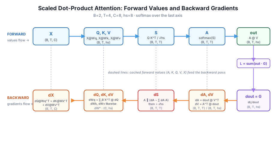
That picture is the whole lesson on one page. Now we derive each backward arrow, right to left, in exactly the order the code runs.

Step 1: Through the Value Multiply, dA and dValue#

The last forward operation was out = A @ V, a batched matrix multiply where, for each item in the batch, $A$ is (T, T) and $V$ is (T, hs). This is the same matrix-multiply rule you know from dense layers, applied per batch element. For a product $\text{out} = A V$, the gradient on each factor is the incoming gradient multiplied by the other factor, transposed:

The only new detail versus a 2D layer is that these are batched, so “transpose” means swapping the last two axes, V.transpose(0, 2, 1), not V.T (which would also flip the batch axis and give the wrong shape). Check the shapes: dout is (B, T, hs) and $V^\top$ is (B, hs, T), so dA is (B, T, T), matching A. And $A^\top$ is (B, T, T) times dout (B, T, hs) gives dValue of shape (B, T, hs), matching V.

dA = dout @ V.transpose(0, 2, 1)   # (B, T, T)   dout @ V^T
dValue = A.transpose(0, 2, 1) @ dout   # (B, T, hs)  A^T @ dout

dValue is already a finished gradient on a forward tensor; it will flow all the way back to dWv and dX later. dA, the gradient on the attention weights, is the input to the trickiest step in the whole course: the softmax.

Step 2: Through the Softmax, dS#

Each row of $A$ is a softmax of the matching row of $S$. Softmax is not elementwise, so its gradient is not a simple elementwise multiply. Within one row, changing a single score $S_j$ changes every output probability $A_i$, because the normalizing sum in the denominator ties them together. For a single row, the derivative of output $A_i$ with respect to input $S_j$ is the softmax Jacobian

where $\delta_{ij}$ is 1 when $i = j$ and 0 otherwise. Written as a matrix over one row, that Jacobian is

a dense (T, T) matrix. The diagonal term $A_i(1 - A_i)$ is how a probability responds to its own score; the off-diagonal term $-A_i A_j$ is how it is pulled down when a competing score rises. The gradient of the loss with respect to the row of scores is this Jacobian applied to the incoming row gradient: $dS_{\text{row}} = J^\top \, dA_{\text{row}}$. Because $J$ is symmetric here, working that product out entry by entry collapses to a compact vectorized form that needs no explicit (T, T) Jacobian:

Read it as: each score’s gradient is its probability times its own incoming gradient, minus the average incoming gradient weighted by the row’s probabilities. That subtracted term is shared by every entry in the row, which is exactly the coupling the off-diagonal Jacobian encodes. In NumPy the whole thing is one line, broadcast over every row of every batch at once by summing over the last axis with keepdims:

dS = A * (dA - np.sum(dA * A, axis=-1, keepdims=True))   # (B, T, T)

Step 3: Through the Scale and the Scores, dS_scaled, dQuery, dKey#

Recall the forward scaling S = Q @ K.transpose(0, 2, 1) / np.sqrt(hs). Dividing by a constant $\sqrt{hs}$ is a linear operation, so its backward is just the same division applied to the gradient:

dS_scaled = dS / np.sqrt(hs)       # (B, T, T)

Now the unscaled scores are another batched matrix multiply, $S_{\text{raw}} = Q K^\top$, with $Q$ shaped (T, hs) and $K^\top$ shaped (hs, T) per batch element. Apply the same matrix-multiply rule as in Step 1, being careful about which factor is transposed. Differentiating $Q K^\top$:

The dQuery line reads directly: dS_scaled is (B, T, T) and K is (B, T, hs), giving (B, T, hs) to match Q. The dKey line needs the batched transpose of dS_scaled first, because $K$ sits on the right of the product as $K^\top$; transposing the score gradient and multiplying by Q recovers a gradient of shape (B, T, hs) that matches K.

dQuery = dS_scaled @ K                   # (B, T, hs)
dKey = dS_scaled.transpose(0, 2, 1) @ Q   # (B, T, hs)

A quick intuition check: dS_scaled measures how the loss wants each score $S_{ij}$ to move, and a score is the dot product of query $i$ with key $j$. So the gradient on query $i$ is a weighted sum of the keys (weighted by how much each of its scores should change), and symmetrically the gradient on key $j$ is a weighted sum of the queries. The two transposes encode exactly that symmetry.

Step 4: Back to the Parameters and Input, dWq, dWk, dWv, dX#

We now have dQuery, dKey, and dValue, the gradients on the three projected tensors. Each came from a projection like Q = X @ Wq, a matrix multiply of X (B, T, C) by a shared weight Wq (C, hs). The weight is shared across the batch, so its gradient sums the per-item contributions. For each batch element the local rule gives $X^\top dQuery$ of shape (C, hs); summing over the batch axis collapses those into one (C, hs) gradient that matches Wq:

dWq = np.sum(X.transpose(0, 2, 1) @ dQuery, axis=0)   # (C, hs)
dWk = np.sum(X.transpose(0, 2, 1) @ dKey, axis=0)   # (C, hs)
dWv = np.sum(X.transpose(0, 2, 1) @ dValue, axis=0)   # (C, hs)

Finally, X fed all three projections, so gradient flows back to it along three paths and they add. From Q = X @ Wq the input gradient is $dQuery \, W_q^\top$, and likewise for the key and value paths:

Here Wq is a plain (C, hs) matrix shared over the batch, so Wq.T is (hs, C) and dQuery @ Wq.T broadcasts cleanly over the batch to give (B, T, C), matching X. Summing the three contributions is the multivariate chain rule: when one quantity influences the loss through several routes, its gradient is the sum over those routes.

dX = dQuery @ Wq.T + dKey @ Wk.T + dValue @ Wv.T   # (B, T, C)

Collect the whole backward pass into one function and confirm every gradient has the shape of the quantity it belongs to.

def attention_backward(dout, cache):
    X, Wq, Wk, Wv, Q, K, V, A = cache

    dA = dout @ V.transpose(0, 2, 1)            # (B, T, T)
    dValue = A.transpose(0, 2, 1) @ dout            # (B, T, hs)

    # softmax backward, applied independently to each row
    dS = A * (dA - np.sum(dA * A, axis=-1, keepdims=True))   # (B, T, T)
    dS_scaled = dS / np.sqrt(hs)                # (B, T, T)

    dQuery = dS_scaled @ K                          # (B, T, hs)
    dKey = dS_scaled.transpose(0, 2, 1) @ Q       # (B, T, hs)

    dWq = np.sum(X.transpose(0, 2, 1) @ dQuery, axis=0)   # (C, hs)
    dWk = np.sum(X.transpose(0, 2, 1) @ dKey, axis=0)   # (C, hs)
    dWv = np.sum(X.transpose(0, 2, 1) @ dValue, axis=0)   # (C, hs)

    dX = dQuery @ Wq.T + dKey @ Wk.T + dValue @ Wv.T      # (B, T, C)
    return dWq, dWk, dWv, dX

dWq, dWk, dWv, dX = attention_backward(dout, cache)
print("dWq:", dWq.shape, " dWk:", dWk.shape, " dWv:", dWv.shape)
print("dX:", dX.shape)

dWq: (8, 8)  dWk: (8, 8)  dWv: (8, 8)
dX: (2, 4, 8)

Every parameter gradient is (C, hs) = (8, 8), matching its weight, and dX is (2, 4, 8), matching the input. The shapes are right. But shapes only prove the plumbing lines up, not that the numbers are correct. For that we need the gradient check.

Proving It: A Numerical Gradient Check#

The definition of a derivative gives a way to estimate any gradient without calculus at all: nudge one number up by a tiny $\epsilon$, nudge it down by $\epsilon$, see how much the loss $L$ moved, and divide. This central finite difference is accurate to order $\epsilon^2$:

If our analytic backward pass is correct, the numerical estimate must agree with it for every entry of every parameter and for X. We measure agreement with the max relative error over all entries: the largest, across the tensor, of $|a - n| \, / \, \max(|a|, |n|)$, where $a$ is analytic and $n$ is numerical. In float64 with $\epsilon = 10^{-5}$, a correct gradient lands around $10^{-6}$ or smaller; anything like $10^{-2}$ means a real bug.

def numerical_grad(param):
    eps = 1e-5
    grad = np.zeros_like(param)
    it = np.nditer(param, flags=["multi_index"])
    while not it.finished:
        idx = it.multi_index
        original = param[idx]
        param[idx] = original + eps
        Lp = loss_from_out(attention_forward(X, Wq, Wk, Wv)[0])
        param[idx] = original - eps
        Lm = loss_from_out(attention_forward(X, Wq, Wk, Wv)[0])
        param[idx] = original          # always restore the entry
        grad[idx] = (Lp - Lm) / (2 * eps)
        it.iternext()
    return grad

def max_rel_err(analytic, numeric):
    denom = np.maximum(np.abs(analytic), np.abs(numeric)) + 1e-12
    return np.max(np.abs(analytic - numeric) / denom)

print("max relative error (analytic vs. numerical):")
print("  dWq:", max_rel_err(dWq, numerical_grad(Wq)))
print("  dWk:", max_rel_err(dWk, numerical_grad(Wk)))
print("  dWv:", max_rel_err(dWv, numerical_grad(Wv)))
print("  dX :", max_rel_err(dX,  numerical_grad(X)))

max relative error (analytic vs. numerical):
  dWq: 1.4008950364789722e-07
  dWk: 3.4212993729037537e-08
  dWv: 4.2107753701537897e-10
  dX : 1.517927265799911e-09

Every error is between $10^{-7}$ and $10^{-10}$, far below the $10^{-4}$ threshold that separates “correct” from “buggy.” That is the proof: the analytic backward pass, including the subtle softmax Jacobian, computes the same gradients that a brute-force perturbation of the loss produces. Run the whole script a second time and the numbers are byte-for-byte identical, because the seed fixes every random draw and the finite-difference loop is deterministic. dWv and dX are the smallest errors because their gradients flow through the fewest nonlinear steps; dWq is largest because it flows through the full softmax coupling, yet even it is essentially perfect.

Practice Exercises#

Try these before checking the hints. They reuse attention_forward, attention_backward, loss_from_out, numerical_grad, and the tensors defined above.

Exercise 1: Break the Softmax on Purpose#

Replace the softmax backward line with the naive (wrong) version dS = dA * A, which drops the $-\sum_k dA_k A_k$ correction term. Recompute dWq and gradient-check it. Confirm the max relative error explodes, then restore the correct line.

# Your code here: temporarily use dS = dA * A inside a copy of attention_backward,
# recompute dWq, and print max_rel_err(dWq_wrong, numerical_grad(Wq))

Exercise 2: Check the Softmax Jacobian Directly#

For a single row a = A[0, 0] (a length-T probability vector), build the full Jacobian matrix $J = \operatorname{diag}(a) - a a^\top$ explicitly with np.diag and an outer product, then confirm that applying it to a random row gradient, J @ g, equals the vectorized formula a * (g - (g * a).sum()).

a = A[0, 0]                      # one softmax row, shape (T,)
g = np.random.randn(T)           # a pretend incoming row gradient dA_row
# Your code here: build J, compare J @ g to the vectorized dS formula

Exercise 3: Gradient-Check a Single dWk Entry by Hand#

Instead of the full-tensor numerical_grad, perturb just Wk[0, 0] by $\pm \epsilon$, estimate that one partial derivative with the central difference, and compare it to dWk[0, 0]. This is the smallest possible gradient check and the fastest way to sanity-test one entry.

eps = 1e-5
# Your code here: perturb Wk[0, 0] up and down, recompute the loss each time,
# form the central difference, and compare to dWk[0, 0]

Summary#

You derived and verified the complete backward pass through scaled dot-product self-attention, the single hardest piece of building a transformer by hand. Let’s review.

Key Concepts#

The Setup

• Cache the forward tensors (X, Q, K, V, A) so the backward pass can reuse them
• Use tiny dims and float64 so a finite-difference check is fast and trustworthy
• Define a scalar loss $L = \sum \text{out} \cdot G$ so the upstream gradient is exactly dout = G

The Backward Pass, In Order

• dA = dout @ V^T, dValue = A^T @ dout — the matrix-multiply rule through out = A @ V (batched transpose on the last two axes)
• dS = A * (dA - sum(dA * A, axis=-1, keepdims=True)) — the softmax Jacobian $\operatorname{diag}(A) - A A^\top$ applied per row
• dS_scaled = dS / sqrt(hs) — the constant scale passes straight through
• dQuery = dS_scaled @ K, dKey = dS_scaled^T @ Q — the matrix-multiply rule through $Q K^\top$
• dWq/dWk/dWv = sum over batch of X^T @ dQuery/dKey/dValue — shared weights sum their gradient over the batch
• dX = dQuery @ Wq^T + dKey @ Wk^T + dValue @ Wv^T — three projection paths add at the input

Proving It

• Every gradient has the same shape as its quantity; a shape mismatch is a bug you can catch before running
• A central finite difference $(L(\theta+\epsilon) - L(\theta-\epsilon)) / 2\epsilon$ estimates any gradient with no calculus
• Real max relative errors were 1e-7 (dWq) down to 1e-9–1e-10 (dX, dWv), all far below the 1e-4 bar, and identical on re-run

Why This Matters#

The softmax Jacobian you implemented here is not a detail; it is the mathematical heart of what makes attention trainable. Everything else in a transformer, the projections, the residual adds, the layer norms, the output head, reuses gradient rules you already knew. Attention’s one new idea, differentiating through a normalized similarity, is the step that lets gradient descent reshape which positions attend to which. When you later watch your mini-GPT learn that a letter should attend to the letters that predict it, this backward pass is the machinery doing the learning.

Just as important, you now know how to prove a hand-derived gradient rather than hope it is right. The perturb-and-compare gradient check is the professional standard for any custom layer: whenever you write a backward pass a framework did not give you, this is how you verify it before trusting it in a training run. A wrong gradient does not crash; it quietly trains the wrong model. The check you wrote is the difference between guessing and knowing.

Continue Building Your Skills#

You have every gradient for a single attention head, derived by hand and confirmed against the numerical truth. What remains is to package it. In the next lesson, the module’s guided project, you will fold this forward and backward pass into one reusable SelfAttention layer class with forward and backward methods, an object that holds its own Wq, Wk, Wv, stashes its cache during the forward call, and hands back dWq, dWk, dWv, and dX during the backward call, gradient-checked end to end. That class is the building block you will stack into multi-head attention and, eventually, the full transformer block that your char-level GPT is made of. The hard derivation is behind you; from here on, attention is a component you can drop in and trust.