Lesson 5 - Guided Project: A Self-Attention Layer Class

Welcome to the Guided Project#

Across this module you built self-attention one operation at a time: the query, key, and value projections; scaled dot-product attention and why the $1/\sqrt{hs}$ scaling is not optional; how to read the attention matrix; and finally the full backward pass, derived by hand and checked against a numerical gradient. In this guided project you stop treating those pieces as loose functions and package them into a single object: a SelfAttention class with a forward and a backward method, holding its own parameters and gradients.

This class is not throwaway demo code. It is the exact building block you will stack in Module 3 (multiple heads side by side), Module 5 (a full transformer block), and Modules 6 and 7 (the causal, trainable GPT). Getting it clean and provably correct now means every later module inherits a component you already trust. So the project ends where every serious layer should: a float64 gradient check that compares the analytic gradients to finite differences, and a short manual gradient-descent run that shows a real loss going down.

By the end of this project, you will be able to:

• Structure a neural network layer as a class that stores its parameters, its forward cache, and its gradients
• Implement forward(X) so it computes attention and caches exactly what backward will need
• Implement backward(dout) so it returns dX and stores self.dWq, self.dWk, self.dWv
• Gradient-check the whole class in float64, reporting max relative errors for Wq, Wk, Wv, and X
• Run a handful of gradient-descent steps on the class and confirm a scalar loss decreases

This project assumes you have followed the earlier lessons in this module, especially the backward-pass derivation in Lesson 4. You only need numpy (version 2.x is fine) — no PyTorch, no GPU, no API key.

Stage 1: The Class Skeleton#

A layer needs three kinds of state: its parameters (the weights it learns), a cache (forward values the backward pass will reuse), and its gradients (filled in by backward). We set all three up in __init__, along with the two numbers that define the layer’s shape: the input width C and the head size hs. The three projection matrices Wq, Wk, Wv each have shape (C, hs) — they map a C-dimensional token vector to an hs-dimensional query, key, or value.

We initialize the weights small (* 0.02, the standard transformer init) and seed the draw so the class is reproducible. The cache starts as None and the gradient attributes start unset; forward and backward will populate them.

import numpy as np

def softmax(x, axis=-1):
    x = x - x.max(axis=axis, keepdims=True)   # stable: subtract row max
    e = np.exp(x)
    return e / e.sum(axis=axis, keepdims=True)

class SelfAttention:
    """A single self-attention head as a reusable NumPy layer."""

    def __init__(self, C, hs, seed=42):
        self.C = C                    # input width (features per token)
        self.hs = hs                  # head size (query/key/value width)
        rng = np.random.default_rng(seed)
        self.Wq = rng.standard_normal((C, hs)) * 0.02   # (C, hs)
        self.Wk = rng.standard_normal((C, hs)) * 0.02   # (C, hs)
        self.Wv = rng.standard_normal((C, hs)) * 0.02   # (C, hs)
        self.cache = None             # filled by forward, read by backward
        self.dWq = self.dWk = self.dWv = None           # parameter gradients

layer = SelfAttention(C=8, hs=4)
print("C, hs:", layer.C, layer.hs)
print("Wq/Wk/Wv shapes:", layer.Wq.shape, layer.Wk.shape, layer.Wv.shape)
print("cache starts empty:", layer.cache)

C, hs: 8 4
Wq/Wk/Wv shapes: (8, 4) (8, 4) (8, 4)
cache starts empty: None

The skeleton holds exactly what a layer must remember about itself: its shape (C = 8, hs = 4), its three (8, 4) weight matrices, and empty slots for the cache and gradients. Nothing has flowed through it yet. Notice that __init__ takes only C and hs — the batch size B and sequence length T are not baked into the layer. That is deliberate: the same object must work on a (2, 5, 8) input today and a (32, 32, 64) input when we scale up, so the layer commits only to widths, never to how many tokens you feed it.

Stage 2: The forward Method#

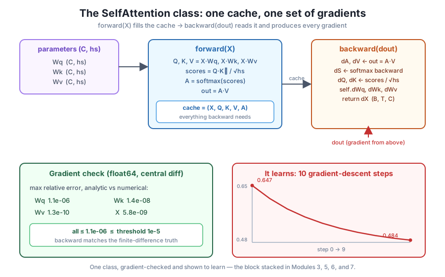
Now we give the class a forward(X) method. It is the scaled dot-product attention you derived earlier, with one addition that matters enormously for what comes next: it caches every value the backward pass will need. Concretely, forward computes Q, K, V, the scaled scores, the softmax weights A, and the output out — then stores (X, Q, K, V, A) on self.cache before returning out.

Why those five and not others? The backward pass needs the input X (to form the weight gradients), the values V and the attention weights A (to differentiate out = A @ V), and Q and K (to differentiate the scores). Everything else can be recomputed cheaply or is not needed. Here is the class with forward added, run on a real (2, 5, 8) input.

import numpy as np

def softmax(x, axis=-1):
    x = x - x.max(axis=axis, keepdims=True)
    e = np.exp(x)
    return e / e.sum(axis=axis, keepdims=True)

class SelfAttention:
    """A single self-attention head as a reusable NumPy layer."""

    def __init__(self, C, hs, seed=42):
        self.C = C
        self.hs = hs
        rng = np.random.default_rng(seed)
        self.Wq = rng.standard_normal((C, hs)) * 0.02
        self.Wk = rng.standard_normal((C, hs)) * 0.02
        self.Wv = rng.standard_normal((C, hs)) * 0.02
        self.cache = None
        self.dWq = self.dWk = self.dWv = None

    def forward(self, X):
        Q = X @ self.Wq                                  # (B, T, hs)
        K = X @ self.Wk                                  # (B, T, hs)
        V = X @ self.Wv                                  # (B, T, hs)
        scores = Q @ K.transpose(0, 2, 1) / np.sqrt(self.hs)   # (B, T, T)
        A = softmax(scores, axis=-1)                     # (B, T, T)
        out = A @ V                                       # (B, T, hs)
        self.cache = (X, Q, K, V, A)                      # everything backward needs
        return out

np.random.seed(42)
B, T, C, hs = 2, 5, 8, 4
X = np.random.randn(B, T, C).astype(np.float64)          # (2, 5, 8)
layer = SelfAttention(C, hs)
out = layer.forward(X)

X_c, Q_c, K_c, V_c, A_c = layer.cache
print("X.shape    :", X.shape)
print("Q,K,V      :", Q_c.shape, K_c.shape, V_c.shape)
print("A (weights):", A_c.shape, "| rows sum to 1:", np.allclose(A_c.sum(-1), 1.0))
print("out.shape  :", out.shape)

X.shape    : (2, 5, 8)
Q,K,V      : (2, 5, 4) (2, 5, 4) (2, 5, 4)
A (weights): (2, 5, 5) | rows sum to 1: True
out.shape  : (2, 5, 4)

Every shape lands where the module’s conventions promise. The (2, 5, 8) input projects through the (8, 4) matrices to give Q, K, V of shape (2, 5, 4) = (B, T, hs). The scores Q K^\top / \sqrt{hs} compare all five queries against all five keys, giving the (2, 5, 5) = (B, T, T) grid, and softmax over the last axis makes each row a probability distribution — confirmed by rows sum to 1: True. The output out = A @ V is back to (2, 5, 4): one refined vector per position. Critically, self.cache now holds the five arrays backward will read. The forward pass is the same math as before; the only new idea is that it deliberately leaves a trail.

Stage 3: The backward Method#

This is where the class earns its keep. The backward(dout) method takes the gradient of the loss with respect to the layer’s output and walks it back through every operation — in the exact reverse order of forward — producing the gradient with respect to the input (dX, which it returns) and the gradients with respect to the parameters (self.dWq, self.dWk, self.dWv, which it stores for the optimizer to use). Each line is one step from the Lesson 4 derivation, now reading its inputs from self.cache.

Walk it top to bottom and you are walking the forward pass in reverse:

• out = A @ V gives dA = dout @ V^T and dValue = A^T @ dout.
• A = softmax(scores) gives the row-wise softmax gradient dS = A * (dA - sum(dA * A)).
• scores = Q K^T / sqrt(hs) gives dscores = dS / sqrt(hs), then dQuery = dscores @ K and dKey = dscores^T @ Q.
• Q, K, V = X @ Wq, X @ Wk, X @ Wv gives the parameter gradients (sum the C x hs contributions over batch and time) and dX from all three projection paths.

import numpy as np

def softmax(x, axis=-1):
    x = x - x.max(axis=axis, keepdims=True)
    e = np.exp(x)
    return e / e.sum(axis=axis, keepdims=True)

class SelfAttention:
    """A single self-attention head as a reusable NumPy layer."""

    def __init__(self, C, hs, seed=42):
        self.C = C
        self.hs = hs
        rng = np.random.default_rng(seed)
        self.Wq = rng.standard_normal((C, hs)) * 0.02
        self.Wk = rng.standard_normal((C, hs)) * 0.02
        self.Wv = rng.standard_normal((C, hs)) * 0.02
        self.cache = None
        self.dWq = self.dWk = self.dWv = None

    def forward(self, X):
        Q = X @ self.Wq
        K = X @ self.Wk
        V = X @ self.Wv
        scores = Q @ K.transpose(0, 2, 1) / np.sqrt(self.hs)
        A = softmax(scores, axis=-1)
        out = A @ V
        self.cache = (X, Q, K, V, A)
        return out

    def backward(self, dout):
        X, Q, K, V, A = self.cache
        # out = A @ V
        dA = dout @ V.transpose(0, 2, 1)                        # (B, T, T)
        dValue = A.transpose(0, 2, 1) @ dout                        # (B, T, hs)
        # A = softmax(scores), row-wise
        dS = A * (dA - (dA * A).sum(axis=-1, keepdims=True))    # (B, T, T)
        # scores = Q K^T / sqrt(hs)
        dscores = dS / np.sqrt(self.hs)                         # (B, T, T)
        dQuery = dscores @ K                                        # (B, T, hs)
        dKey = dscores.transpose(0, 2, 1) @ Q                     # (B, T, hs)
        # Q,K,V = X @ Wq, X @ Wk, X @ Wv  (sum the C x hs outer products over B,T)
        self.dWq = np.einsum('btc,bth->ch', X, dQuery)              # (C, hs)
        self.dWk = np.einsum('btc,bth->ch', X, dKey)              # (C, hs)
        self.dWv = np.einsum('btc,bth->ch', X, dValue)              # (C, hs)
        dX = dQuery @ self.Wq.T + dKey @ self.Wk.T + dValue @ self.Wv.T   # (B, T, C)
        return dX

np.random.seed(42)
B, T, C, hs = 2, 5, 8, 4
X = np.random.randn(B, T, C).astype(np.float64)
layer = SelfAttention(C, hs)
out = layer.forward(X)

dout = np.random.randn(*out.shape)          # a pretend gradient from the layer above
dX = layer.backward(dout)
print("dout.shape :", dout.shape)
print("dWq/dWk/dWv:", layer.dWq.shape, layer.dWk.shape, layer.dWv.shape)
print("dX.shape   :", dX.shape)

dout.shape : (2, 5, 4)
dWq/dWk/dWv: (8, 4) (8, 4) (8, 4)
dX.shape   : (2, 5, 8)

The shapes are the immediate sanity check, and they all match: a gradient always has the same shape as the thing it belongs to. dX is (2, 5, 8) like the input X, and each of dWq, dWk, dWv is (8, 4) like its weight matrix. The np.einsum('btc,bth->ch', X, dQuery) line is worth reading slowly: it sums the outer product of X (C features) and dQuery (hs outputs) over both the batch axis b and the time axis t, exactly as X^T @ dQuery would for a 2D input, but handled cleanly across the extra batch dimension. Shapes matching is necessary but not sufficient, though — a transpose in the wrong place can still pass the shape test. That is why the next stage proves correctness numerically.

Stage 4: Prove the Class Is Correct#

A backward pass you cannot verify is a backward pass you cannot trust. We prove this one two ways: a gradient check (do the analytic gradients match finite differences?) and a learning check (does a real loss actually go down when we descend those gradients?).

Gradient Check#

The idea is the definition of a derivative. Nudge one entry of a parameter by $\pm \epsilon$, measure how much a scalar loss changes, and divide — that finite difference must match the analytic gradient:

We use a simple scalar loss $L = \sum (\text{out} \odot G)$ for a fixed random matrix $G$, because then the analytic gradient flowing into backward is just dout = G. We run the check in float64 (finite differences are numerically delicate; single precision would swamp the signal with rounding noise) and report the max relative error across every entry of Wq, Wk, Wv, and X.

def scalar_loss(out, G):
    return np.sum(out * G)

def rel_err(a, b):
    return np.max(np.abs(a - b) / np.maximum(1e-12, np.abs(a) + np.abs(b)))

def numeric_grad(layer, X, P, G, eps=1e-6):
    """Central-difference gradient of scalar_loss w.r.t. every entry of array P."""
    g = np.zeros_like(P)
    it = np.nditer(P, flags=['multi_index'])
    while not it.finished:
        idx = it.multi_index
        old = P[idx]
        P[idx] = old + eps; lp = scalar_loss(layer.forward(X), G)
        P[idx] = old - eps; lm = scalar_loss(layer.forward(X), G)
        P[idx] = old
        g[idx] = (lp - lm) / (2 * eps)
        it.iternext()
    return g

np.random.seed(42)
B, T, C, hs = 2, 5, 8, 4
X = np.random.randn(B, T, C).astype(np.float64)
layer = SelfAttention(C, hs)
G = np.random.randn(B, T, hs)               # fixed upstream gradient

layer.forward(X)
dX = layer.backward(G)                       # analytic dWq/dWk/dWv and dX
num_Wq = numeric_grad(layer, X, layer.Wq, G)
num_Wk = numeric_grad(layer, X, layer.Wk, G)
num_Wv = numeric_grad(layer, X, layer.Wv, G)
num_X  = numeric_grad(layer, X, X, G)
layer.forward(X); dX = layer.backward(G)     # recompute analytic dX after perturbing X

print("max rel err  Wq:", rel_err(layer.dWq, num_Wq))
print("max rel err  Wk:", rel_err(layer.dWk, num_Wk))
print("max rel err  Wv:", rel_err(layer.dWv, num_Wv))
print("max rel err   X:", rel_err(dX, num_X))

max rel err  Wq: 1.1223224453603012e-06
max rel err  Wk: 1.3695050922138893e-08
max rel err  Wv: 1.2792434743768677e-10
max rel err   X: 5.838655882581577e-09

Every max relative error is around $10^{-6}$ or far smaller — the largest, on Wq, is 1.1e-06, comfortably under the 1e-5 bar we set for “the backward pass is correct.” Read the sizes: dWv (1.3e-10) is the most accurate because it flows through only one operation (out = A @ V), while dWq accumulates a little more finite-difference noise because its gradient threads all the way back through the softmax. All four are tiny, which is the numerical proof that backward implements the true derivative of forward.

It Learns#

Matching finite differences proves the gradients are correct; the final check proves they are useful. We pick a fixed random target Y, define a mean-squared-error loss between the layer’s output and Y, and take ten manual gradient-descent steps — each one a forward, a backward, and a subtraction of lr times each parameter gradient. If the gradients truly point downhill, the printed loss must fall.

np.random.seed(0)
B, T, C, hs = 2, 5, 8, 4
X = np.random.randn(B, T, C)
Y = np.random.randn(B, T, hs)               # a fixed random target to fit
lay = SelfAttention(C, hs)
lr = 0.5

for step in range(10):
    o = lay.forward(X)
    loss = 0.5 * np.mean((o - Y) ** 2)
    dout = (o - Y) / o.size                  # gradient of the MSE loss
    lay.backward(dout)
    lay.Wq -= lr * lay.dWq
    lay.Wk -= lr * lay.dWk
    lay.Wv -= lr * lay.dWv
    print(f"step {step:2d}  loss {loss:.4f}")

step  0  loss 0.6470
step  1  loss 0.6077
step  2  loss 0.5770
step  3  loss 0.5530
step  4  loss 0.5340
step  5  loss 0.5190
step  6  loss 0.5070
step  7  loss 0.4974
step  8  loss 0.4897
step  9  loss 0.4835

The loss falls monotonically from 0.6470 to 0.4835 across ten steps — every single step lower than the last. That is the whole training loop of a real network in miniature: forward, compute a loss, backward, nudge the parameters against their gradients, repeat. A single attention head cannot perfectly fit a random target (it has limited capacity), so the loss levels off rather than reaching zero, but the steady, gap-free descent is exactly the behavior correct gradients produce. Run this entire lesson a second time: because every random draw is seeded, you get byte-for-byte identical errors and losses — this course has no nondeterminism to hide behind.

Practice Exercises#

Try these before checking the hints. They reuse the SelfAttention class and the setup you built above.

Exercise 1: Gradient-Check a Bigger Layer#

Rerun the gradient check with a larger configuration — say B, T, C, hs = 3, 7, 16, 8 — and confirm the max relative errors are still under 1e-5. A correct backward pass should not care about the sizes.

# Your code here: rebuild X, layer, G with the larger shapes and re-run numeric_grad

Exercise 2: Verify the Loss Really Needs All Three Gradients#

In the “it learns” loop, comment out the update to Wv (keep updating only Wq and Wk) and rerun. Does the loss still fall, and does it reach as low as 0.4835?

# Your code here: update only Wq and Wk each step; leave Wv frozen

Exercise 3: Add a zero_grad Method#

Real training loops reset gradients between steps. Add a method zero_grad(self) that sets self.dWq, self.dWk, self.dWv back to None (or to zero arrays), and call it at the top of the training loop. Confirm the loss sequence is unchanged.

# Your code here: define SelfAttention.zero_grad and call it each step

Summary#

You turned a module’s worth of loose functions into one reusable, provably correct component. Let’s review what you built.

Key Concepts#

The Class Design

• __init__(C, hs) stores the layer’s shape and its three (C, hs) projection matrices Wq, Wk, Wv, initialized small (* 0.02) and seeded
• The layer commits only to widths (C, hs), never to B or T, so the same object works on any batch size or sequence length
• Three kinds of state live on self: parameters, a forward cache, and gradients

forward and backward

• forward(X) computes Q, K, V, scaled scores, softmax A, and out, then caches (X, Q, K, V, A) — exactly what backward needs
• backward(dout) walks the cache in reverse: dA/dValue, softmax-backward dS, dscores, dQuery/dKey, the parameter grads dWq/dWk/dWv, and the returned dX
• A gradient always matches the shape of what it belongs to: dX like X, each dW like its W

Proving Correctness

• A float64 central-difference gradient check gave max relative errors from 1.1e-06 (Wq) down to 1.3e-10 (Wv) — all under the 1e-5 bar
• A ten-step manual gradient-descent run drove a real MSE loss monotonically from 0.6470 to 0.4835, confirming the gradients point downhill
• Everything is seeded and byte-for-byte reproducible on a second run

Why This Matters#

This class is the first component in the course you will genuinely reuse rather than rebuild. Module 3 instantiates several of these and runs them in parallel to make multi-head attention; Module 5 drops one inside a transformer block alongside a feed-forward network and layer norm; Modules 6 and 7 add a causal mask to forward and train stacks of them into a working GPT. Because you gradient-checked it here, none of those modules has to re-derive or re-verify the attention math — they inherit a block that is already known to be correct.

More broadly, the forward-caches / backward-reads-the-cache pattern is the shape of every layer in every deep-learning framework. You now know exactly what a Module or Layer object is hiding: parameters, a cache, gradients, and two methods that are careful reverses of each other. That understanding is what lets you debug a real transformer instead of treating it as a black box.

Continue Building Your Skills#

You have a single, trustworthy attention head packaged as a class — the atom of every model ahead. In the next module, Multi-Head Attention, you will discover why one head is not enough: a single set of Wq, Wk, Wv can only learn one kind of relationship at a time, but language needs many (who did what, what refers to what, what comes next). You will run several SelfAttention heads side by side over different slices of the model width, concatenate their outputs, and mix them with an output projection — turning today’s one head into the parallel, multi-perspective attention that real transformers use. Keep this gradient-checked class close; Module 3 is, quite literally, four of them working at once.