Lesson 1 - Residual Connections

Welcome to Residual Connections#

You have spent the last few modules building the pieces of a transformer: token and position embeddings, scaled dot-product attention, and multi-head attention. Each of those is a sublayer, a block that takes a (B, T, C) activation and returns another (B, T, C) activation. To build a real GPT you need to stack many of these on top of each other, a dozen or more in a full model. And the moment you stack them naively, training breaks: the gradient that has to travel from the loss all the way back to the first layer shrinks to almost nothing on the way, and the early layers stop learning.

This lesson introduces the deceptively simple fix that every transformer relies on: the residual connection, also called a skip connection. Instead of feeding a sublayer’s output straight into the next block, you add the sublayer’s input back onto its output: out = x + sublayer(x). The forward pass barely changes. The backward pass changes everything.

By the end of this lesson, you will be able to:

• Write a residual connection as out = x + sublayer(x) and explain the shape constraint it imposes
• Derive the backward pass dx = dout + df and explain why the + x path has a local derivative of exactly 1
• Explain how that identity path gives every layer a direct gradient route to the loss
• Build a NumPy demo that measures gradient norm through a deep stack with and without residuals
• Gradient-check the residual backward pass in float64 and confirm it matches a finite difference

You should already be comfortable with the backward pass of a simple network (the chain rule, naming a gradient dX after the quantity X) and with the (B, T, C) activation convention we use throughout this course. Let’s begin.

The Vanishing-Gradient Problem, Revisited#

Back in Module 1 you saw why plain recurrent networks struggle on long sequences: the gradient has to pass through the same operation once per timestep, and each pass multiplies it by a factor. If that factor is a little less than 1, the gradient decays geometrically, and after many steps it is effectively zero. The network cannot learn long-range dependencies because no learning signal survives the trip back.

A deep stack of sublayers has the exact same disease, just along depth instead of time. Consider what happens to a gradient as it travels backward through $N$ stacked sublayers, where sublayer $i$ computes $x_{i+1} = f_i(x_i)$:

That is a product of $N$ Jacobians. If each one shrinks the gradient by roughly a factor $\gamma < 1$, the whole product scales like $\gamma^{N}$, which races toward zero as the stack gets deep. The early layers, the ones closest to the input, receive a gradient so tiny that their weights never meaningfully update. A 12-layer transformer built this way simply would not train.

We want a way to stack many sublayers without the gradient having to survive a long product of shrinking factors. That is exactly what a residual connection buys us.

The Residual Connection: Forward#

The idea is almost embarrassingly simple. A normal sublayer replaces its input:

A residual sublayer adds to its input instead:

The sublayer $f$ now only has to learn the change it wants to make to x, the residual, rather than reproducing all of x from scratch and then modifying it. If a sublayer has nothing useful to add, it can push $f(x)$ toward zero and the block becomes an identity map, passing x through untouched. That is a much easier default for a deep network to fall back on than learning to copy its input through a nonlinearity.

In code the forward pass is a single addition:

import numpy as np

def residual(x, sublayer):
    # x: (B, T, C);  sublayer maps (B, T, C) -> (B, T, C)
    return x + sublayer(x)

There is one hard requirement hiding in that +: the sublayer’s output must have the same shape as its input, because you are adding them element-wise. This is why every transformer sublayer, attention and the feed-forward network alike, is carefully built to map (B, T, C) to (B, T, C). The residual connection is the reason the model width C stays constant all the way up the stack.

The Residual Connection: Backward#

The forward pass was trivial. The whole payoff is in the backward pass, so let’s derive it carefully.

Our block is $\text{out} = x + f(x)$. We want $\frac{\partial L}{\partial x}$, given the upstream gradient $\text{dout} = \frac{\partial L}{\partial \text{out}}$. Because the output is a sum of two terms, the gradient with respect to x picks up a contribution from each term:

The first term is the local derivative of x with respect to itself, which is exactly 1. The second term is the gradient sent back through the sublayer, which we will call df. So the residual backward pass is:

where df is whatever dout becomes after flowing backward through f. Read that carefully. The upstream gradient dout appears twice on the right: once routed through the sublayer as part of df, and once passed straight through unchanged by the + x path. That straight-through copy is the entire trick.

def residual_backward(dout, df):
    # dout: gradient of the loss wrt the block output  (B, T, C)
    # df:   gradient sent back through the sublayer f    (B, T, C)
    dx = dout + df      # the + x path has local derivative 1
    return dx

Compare this to a plain sublayer, where $\text{out} = f(x)$ and therefore dx = df with no extra term. In the plain case the gradient has only the sublayer route home, and that route shrinks it. In the residual case there is an additional route, the identity path, whose local derivative is 1, so it neither shrinks nor grows the gradient. No matter how much f attenuates its portion, the dout that flows through the + x path arrives at the input intact.

Stack $N$ of these, and the identity paths chain into one continuous highway: the gradient from the loss can reach layer 0 by hopping along the + x connections without ever passing through a single weight matrix. Every layer therefore has a direct gradient path to the loss. That is why the product-of-shrinking-factors problem disappears.

Measuring It: A Real Deep Stack in NumPy#

Talk is cheap; let’s measure the effect. We will build a stack of $N$ sublayers, each a small linear map followed by a tanh. We deliberately scale each linear map so that its Jacobian attenuates the gradient, roughly the way a poorly conditioned deep network would. Then we run the gradient backward through the whole stack two ways, with the residual + x path and without it, and measure the norm of the gradient that finally reaches the input.

Everything is seeded so the run is fully reproducible.

import numpy as np

np.random.seed(42)

C = 16          # feature width
B = 4           # a small batch of vectors
depths = [1, 5, 10, 20]

# A fixed bank of sublayers. Each is a linear map whose Jacobian attenuates the
# gradient (spectral scale ~0.5), followed by a saturating tanh. We reuse the
# SAME weights for every depth so the only thing changing is N and the + x path.
MAX_N = max(depths)
Ws = [np.random.randn(C, C) * (0.5 / np.sqrt(C)) for _ in range(MAX_N)]

def sublayer_forward(x, W):
    z = x @ W
    a = np.tanh(z)
    return a, (x, z)          # cache x and the pre-activation z

def sublayer_backward(dout, cache, W):
    x, z = cache
    dz = dout * (1.0 - np.tanh(z) ** 2)   # local derivative of tanh
    dx = dz @ W.T                         # gradient wrt the sublayer's input
    return dx

Now the stack itself. On the forward pass we either add the input back (x = x + f) or not (x = f). On the backward pass the residual case adds dout straight through (dx = dx + df), while the plain case keeps only df.

def run_stack(N, residual):
    x = np.random.RandomState(0).randn(B, C)   # same input every call
    caches = []
    for i in range(N):
        f, cache = sublayer_forward(x, Ws[i])
        caches.append(cache)
        x = x + f if residual else f           # <-- the residual connection

    dout = np.ones_like(x)                      # upstream gradient of norm sqrt(B*C) = 8
    dx = dout
    for i in reversed(range(N)):
        df = sublayer_backward(dx, caches[i], Ws[i])
        dx = dx + df if residual else df        # <-- + x path passes dout through
    return np.linalg.norm(dx)                   # norm of gradient reaching the input

print(f"{'depth N':>8} | {'no residual':>14} | {'with residual':>14}")
print("-" * 44)
for N in depths:
    g_none = run_stack(N, residual=False)
    g_res = run_stack(N, residual=True)
    print(f"{N:>8} | {g_none:>14.6e} | {g_res:>14.6f}")

Running it prints a real table:

 depth N |    no residual |  with residual
--------------------------------------------
       1 |   2.778871e+00 |       8.671100
       5 |   7.579453e-02 |      14.544574
      10 |   1.856928e-03 |      18.981747
      20 |   8.262664e-07 |      25.643279

Read the two columns. The upstream gradient starts with norm $\sqrt{B \cdot C} = \sqrt{64} = 8.0$ at the output. Without residuals, by the time it reaches the input of a 20-layer stack its norm has collapsed to 8.26e-07, seven orders of magnitude smaller. Those early layers are receiving essentially no signal; they are frozen. With residuals, the same gradient arrives with norm 25.6, comfortably the same order of magnitude it started at. The identity highway kept it alive across all 20 layers.

Run the block a second time and you get byte-for-byte the same table: the fixed seeds make this completely deterministic.

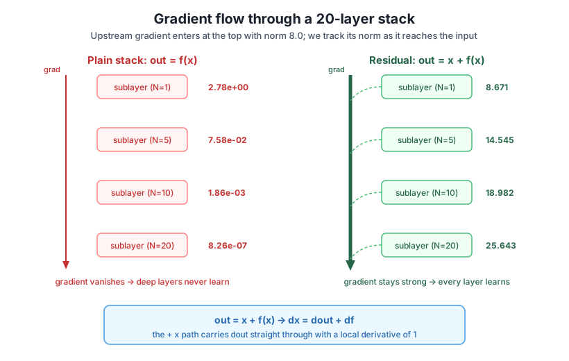
Notice one honest detail in the residual column: the norm does not stay pinned at exactly 8, it drifts upward to 25.6. That mild growth is the sublayer contributions df accumulating along the way, and it is precisely the reason the next lesson adds layer normalization to keep the residual stream’s scale in check. The headline result stands: residuals turn a seven-order-of-magnitude collapse into a small, well-behaved factor.

Proving the Backward Pass Is Correct#

Whenever we write a backward pass in this course, we prove it with a gradient check: compare the analytic gradient to a numerical finite difference in float64 and confirm the max relative error is tiny. Residual connections are no exception, and the check is a nice way to see the dx = dout + df formula hold up numerically.

import numpy as np

rng = np.random.default_rng(42)
C = 8
x = rng.standard_normal((3, C)).astype(np.float64)
W = (rng.standard_normal((C, C)) * (0.5 / np.sqrt(C))).astype(np.float64)

def residual_forward(x):
    z = x @ W
    f = np.tanh(z)
    out = x + f                    # residual connection
    return out, (x, z)

def residual_backward(dout, cache):
    x, z = cache
    df = (dout * (1.0 - np.tanh(z) ** 2)) @ W.T   # gradient through the sublayer
    dx = dout + df                                # + x path adds dout straight through
    return dx

# analytic gradient of L = sum(out) wrt x
out, cache = residual_forward(x)
dout = np.ones_like(out)
dx = residual_backward(dout, cache)

# numerical gradient by central finite differences
eps = 1e-6
num = np.zeros_like(x)
for i in range(x.shape[0]):
    for j in range(x.shape[1]):
        xp = x.copy(); xp[i, j] += eps
        xm = x.copy(); xm[i, j] -= eps
        num[i, j] = (residual_forward(xp)[0].sum() - residual_forward(xm)[0].sum()) / (2 * eps)

rel = np.abs(dx - num) / (np.abs(dx) + np.abs(num) + 1e-12)
print("max relative error:", f"{rel.max():.2e}")
print("dtype:", dx.dtype)

The output confirms the derivation:

max relative error: 5.68e-10
dtype: float64

A max relative error of 5.68e-10, far below our 1e-4 bar, means the analytic dx = dout + df matches the true gradient to nine decimal places. The + x path really does contribute a clean copy of dout, exactly as the derivation claimed. Re-running gives the identical number.

Practice Exercises#

Try each one before opening the hint. They reuse the Ws, run_stack, and gradient-check code from above.

Exercise 1: Weaken the Attenuation#

Change the sublayer scale from 0.5 / np.sqrt(C) to 0.9 / np.sqrt(C) and rebuild the Ws bank, then reprint the table. Does the no-residual column still decay as you go deeper? Does the residual column still stay healthy?

# Your code here: rebuild Ws with the 0.9 scale, then loop over depths again

Exercise 2: Gradient-Check the Two-Sublayer Residual#

Extend the gradient check to a stack of two residual sublayers, out = h + g(h) where h = x + f(x), and confirm the analytic dx still matches the numerical gradient in float64.

# Your code here: chain two residual_forward calls, backprop through both,
# then finite-difference the whole thing

Exercise 3: Report the Preservation Ratio#

For the residual stack, compute the ratio of the input-gradient norm to the starting upstream norm (8.0) at each depth. This single number captures “how much of the gradient survived the trip.”

# Your code here: for N in depths, print run_stack(N, residual=True) / 8.0

Summary#

You added the single most important structural trick for training deep networks, and you proved it works with real numbers. Let’s review.

Key Concepts#

The Idea

• A residual (skip) connection computes out = x + sublayer(x): it adds the input back onto the sublayer’s output instead of replacing it
• The sublayer only has to learn the change to make to x; if it has nothing to add, f(x) -> 0 turns the block into an identity map
• The addition forces the sublayer to preserve shape, which is why the residual stream keeps width C all the way up a transformer

The Backward Pass

• Because out = x + f(x), the gradient splits: dx = dout + df
• The + x path has a local derivative of exactly 1, so it passes dout straight through, unattenuated
• Stacked residuals chain their identity paths into a gradient highway, giving every layer a direct route to the loss

What We Measured

• Through a 20-layer attenuating stack, the plain gradient norm collapsed from 8.0 to 8.26e-07, while the residual gradient norm stayed healthy at 25.6
• The residual backward pass gradient-checked in float64 with max relative error 5.68e-10, far under the 1e-4 bar
• Residuals do not remove the sublayer’s gradient; they add an unattenuated copy of dout on top of it

Why This Matters#

Residual connections are what make depth practical. Before they became standard, networks past a handful of layers were painful or impossible to train, because the gradient vanished on its way back, the same decay you first saw in recurrent networks along the time axis. The + x identity path breaks that decay by giving the gradient a route home that no weight matrix ever shrinks. This is why every real transformer, from a two-layer tutorial model to a frontier-scale system with dozens of layers, wraps each attention block and each feed-forward block in a residual connection. When you assemble the full transformer block later in this module, you will see the residual stream running straight up the middle, with attention and the feed-forward network each adding their contribution to it rather than overwriting it.

Continue Building Your Skills#

You now have the backbone of the transformer block: an identity path that lets the gradient flow freely no matter how deep the model gets. But you also saw the one wrinkle in the residual column of that table, the gradient norm creeping upward as the sublayer contributions pile onto the residual stream. Left unchecked, that drift makes activations grow layer by layer and destabilizes training. The next lesson introduces layer normalization, the companion to the residual connection that re-centers and re-scales each activation vector to keep the residual stream well-behaved. You will build it from scratch in NumPy, derive its backward pass, gradient-check it, and see exactly where it slots into the block relative to the + x path you built today.