Lesson 2 - Layer Normalization

Welcome to Layer Normalization#

In the last lesson you added residual connections so gradients could survive a deep stack of blocks. Residuals keep the gradient path open, but they do nothing about scale: as signals flow through attention, feed-forward layers, and repeated additions, the numbers in each token vector can drift large or small, and a deep model built on drifting activations is miserable to train. The tiny char-level GPT you are building stacks these blocks, so it needs a way to keep every position’s activations at a sane scale from block to block. That job belongs to layer normalization.

Layer norm is a small operation with a deceptively tricky backward pass. The forward direction is four lines of NumPy. The backward direction is where most from-scratch implementations quietly go wrong, because normalizing a vector makes every output depend on every input through the shared mean and variance. This lesson derives that backward pass carefully and then proves it correct with a numerical gradient check.

By the end of this lesson, you will be able to:

• Explain how layer normalization standardizes each token’s features across the feature dimension C
• Contrast layer norm with batch norm and say why layer norm suits transformers
• Implement layernorm_forward with the right cached values for backpropagation
• Derive dgamma, dbeta, and the subtle dx formula, and explain each of its three terms
• Gradient-check the backward pass in float64 and read the max relative errors

You should be comfortable with the mean/variance operations from earlier modules and with the gradient-check pattern from Deep Learning Foundations. Let’s begin.

Normalizing Across the Feature Dimension#

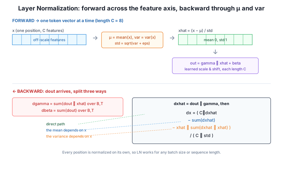
The activations flowing through the model have shape (B, T, C): B sequences, T token positions, and C features per position (C is n_embd, the model width). Layer normalization treats each of those B * T token vectors independently. For a single vector $x$ of length C, it computes the mean and variance over the C features and standardizes:

The small $\epsilon$ inside the square root keeps the division safe when a vector is nearly constant. After standardizing, $\hat{x}$ has mean 0 and standard deviation 1 by construction. But forcing every representation to mean 0 and unit variance is too rigid, so layer norm gives the model two learned vectors, $\gamma$ and $\beta$ (each length C), to scale and shift the normalized values back to whatever distribution the next layer prefers:

Here $\odot$ is element-wise multiplication. If the network wants the raw activations back, it can learn $\gamma = \sqrt{\text{var} + \epsilon}$ and $\beta = \mu$; if it wants pure normalization, it can learn $\gamma = 1, \beta = 0$. The point is that normalization sets a stable starting scale and the learned parameters adjust from there.

Why Layer Norm, Not Batch Norm#

Batch normalization, common in convolutional networks, normalizes each feature across the batch: it computes the mean and variance of one feature over all the examples in the batch. That ties every example’s normalization to the other examples that happen to share its batch, and it needs a running estimate of those statistics for inference. Both properties are awkward for sequence models, where the batch and sequence length change constantly and each position should be treated on its own terms.

Layer normalization sidesteps all of it. Because it normalizes within each token vector, across the feature axis, its computation for one position never touches any other position or any other example. It behaves identically for a batch of 1 or a batch of 512, for a sequence of 8 tokens or 1000, and it needs no running statistics. That per-token independence is exactly what makes deep transformer stacks trainable at any batch or sequence size, which is why the transformer block wraps its sub-layers in layer norm.

The Forward Pass in NumPy#

Here is layernorm_forward. It caches exactly the three values the backward pass will need: the normalized xhat, the scale gamma, and the standard deviation std. We work in float64 throughout so the gradient check later is trustworthy.

import numpy as np

def layernorm_forward(x, gamma, beta, eps=1e-5):
    # x: (B, T, C). Normalize each length-C feature vector on its own.
    mu = x.mean(axis=-1, keepdims=True)          # (B, T, 1)
    var = x.var(axis=-1, keepdims=True)          # (B, T, 1)
    std = np.sqrt(var + eps)                      # (B, T, 1)
    xhat = (x - mu) / std                         # (B, T, C), ~0 mean, ~1 std
    out = gamma * xhat + beta                     # (B, T, C)
    cache = (xhat, gamma, std)
    return out, cache

rng = np.random.default_rng(42)
B, T, C = 2, 4, 8                                  # 2 sequences, 4 tokens, width 8
x = rng.standard_normal((B, T, C)) * 3.0 + 1.5     # deliberately off-scale
gamma = rng.standard_normal(C)                      # learned scale, length C
beta = rng.standard_normal(C)                       # learned shift, length C

out, cache = layernorm_forward(x, gamma, beta)
xhat = cache[0]

print("x shape:   ", x.shape)
print("out shape: ", out.shape)

flat = xhat.reshape(-1, C)                          # 8 token vectors
print("normalized row means (should be ~0):", np.round(flat.mean(axis=1), 9))
print("normalized row stds  (should be ~1):", np.round(flat.std(axis=1), 6))

We deliberately built x with mean around 1.5 and a standard deviation around 3 so there is something real for normalization to fix. Running it:

x shape:    (2, 4, 8)
out shape:  (2, 4, 8)
normalized row means (should be ~0): [-0. -0. -0. -0. -0.  0. -0.  0.]
normalized row stds  (should be ~1): [0.999999 0.999999 0.999999 0.999999 0.999999 0.999997 0.999999 0.999999]

Every one of the eight token vectors comes out with mean 0 and standard deviation 1 (a hair under 1 because of the eps inside the square root). The output keeps the input shape (2, 4, 8), so layer norm slots into the block without disturbing anything downstream. That shape preservation matters: the transformer block wraps layer norm around sub-layers whose input and output shapes must match.

Deriving the Backward Pass#

Now the subtle part. We want the gradients $\frac{\partial L}{\partial \gamma}$, $\frac{\partial L}{\partial \beta}$, and $\frac{\partial L}{\partial x}$, given the upstream gradient dout $= \frac{\partial L}{\partial \text{out}}$ of shape (B, T, C).

The Easy Two: dgamma and dbeta#

The output is $\text{out} = \gamma \odot \hat{x} + \beta$. Both $\gamma$ and $\beta$ have length C and are shared across every position and every example, so a change to $\gamma_i$ affects the output at feature i of all B * T positions. The chain rule therefore sums their contributions over the batch and time axes:

dgamma picks up a factor of $\hat{x}$ because $\gamma$ multiplies $\hat{x}$; dbeta does not, because $\beta$ is just added. Both results have shape (C,), matching the parameters.

The Hard One: dx#

For dx we first push the gradient through the scale-and-shift to reach $\hat{x}$:

Call this dxhat. If $\hat{x}$ depended on $x$ element by element, we would be done: dx would just be dxhat / std. But it does not. Every element $\hat{x}_i = (x_i - \mu)/\sqrt{\text{var}+\epsilon}$ depends on all of $x$, because $\mu$ and $\text{var}$ are computed from the whole vector. Nudging one $x_j$ shifts the mean and the variance, which changes every $\hat{x}_i$. The backward pass has to account for those two coupling paths.

Carefully differentiating $\hat{x} = (x - \mu)/\sqrt{\text{var}+\epsilon}$ with respect to $x$, and letting $\text{std} = \sqrt{\text{var}+\epsilon}$, the three paths (direct, through $\mu$, and through $\text{var}$) collapse into one compact formula:

where each sum runs over the feature axis. Read the three terms inside the parentheses one at a time:

• $C\,\text{dxhat}$ is the direct path: how the loss would move each $x_i$ if the mean and variance were held fixed.
• $-\sum_k \text{dxhat}_k$ is the mean correction. Because $\mu$ is the average of every element, raising one $x_i$ also raises $\mu$, which lowers every $\hat{x}$. This term subtracts the average incoming gradient so the update does not fight the mean it is shifting.
• $-\hat{x}\sum_k \text{dxhat}_k\,\hat{x}_k$ is the variance correction. Changing $x_i$ changes the spread, hence $\text{std}$, hence every $\hat{x}$ in proportion to how far it sits from the mean (that is what the $\hat{x}$ weighting captures). This term removes the component of the gradient that would merely rescale the vector.

Together the two correction terms are what makes layer norm’s backward pass differ from a plain element-wise division. Drop either one and the gradient is subtly wrong in a way that a shape check will never catch, which is exactly why we gradient-check.

Here is layernorm_backward. The feat_axes line sums dgamma and dbeta over the batch and time axes while keeping the feature axis, so both come out length C:

def layernorm_backward(dout, cache):
    xhat, gamma, std = cache
    C = xhat.shape[-1]
    feat_axes = tuple(range(dout.ndim - 1))          # sum over B and T, keep C
    dgamma = np.sum(dout * xhat, axis=feat_axes)     # (C,)
    dbeta = np.sum(dout, axis=feat_axes)             # (C,)
    dxhat = dout * gamma                             # (B, T, C)
    dx = (1.0 / (C * std)) * (
        C * dxhat
        - dxhat.sum(axis=-1, keepdims=True)
        - xhat * (dxhat * xhat).sum(axis=-1, keepdims=True)
    )
    return dx, dgamma, dbeta

The two .sum(axis=-1, keepdims=True) reductions are the mean and variance corrections, and they broadcast back over the feature axis exactly like the forward statistics did.

Gradient-Checking the Backward Pass#

A backward pass that runs without a shape error is not a correct backward pass. To prove correctness we compare each analytic gradient against a numerical one: nudge a single value by a tiny $h$, measure how a scalar loss changes, and divide. For a loss $L$ and any parameter $w$,

We pick the simplest scalar loss whose gradient with respect to out is exactly the upstream dout we already have, namely $L = \sum (\text{dout} \odot \text{out})$. Then the analytic gradients from layernorm_backward must match the finite differences. Everything stays float64 so rounding does not swamp the check.

# scalar loss whose gradient wrt out is exactly dout
def loss_fn(x, gamma, beta):
    out, _ = layernorm_forward(x, gamma, beta)
    return np.sum(dout * out)

def numerical_grad(param, h=1e-6):
    grad = np.zeros_like(param)
    it = np.nditer(param, flags=["multi_index"])
    while not it.finished:
        idx = it.multi_index
        orig = param[idx]
        param[idx] = orig + h; lp = loss_fn(x, gamma, beta)
        param[idx] = orig - h; lm = loss_fn(x, gamma, beta)
        param[idx] = orig
        grad[idx] = (lp - lm) / (2 * h)
        it.iternext()
    return grad

def max_rel_err(a, b):
    return np.max(np.abs(a - b) / np.maximum(1e-12, np.abs(a) + np.abs(b)))

dout = rng.standard_normal((B, T, C))                # pretend upstream gradient
out, cache = layernorm_forward(x, gamma, beta)
dx, dgamma, dbeta = layernorm_backward(dout, cache)
print("dx:", dx.shape, "| dgamma:", dgamma.shape, "| dbeta:", dbeta.shape)

num_dx = numerical_grad(x)
num_dgamma = numerical_grad(gamma)
num_dbeta = numerical_grad(beta)

print("max rel err  dx    :", max_rel_err(dx, num_dx))
print("max rel err  dgamma:", max_rel_err(dgamma, num_dgamma))
print("max rel err  dbeta :", max_rel_err(dbeta, num_dbeta))

Running it prints:

dx: (2, 4, 8) | dgamma: (8,) | dbeta: (8,)
max rel err  dx    : 2.824402011294511e-08
max rel err  dgamma: 1.757852155326469e-09
max rel err  dbeta : 3.4275647975734703e-10

Every gradient agrees with its numerical estimate to a max relative error near $10^{-8}$, far below the $10^{-6}$ we would demand of a float64 check. The three-term dx is correct. Re-run the whole script and the numbers are byte-for-byte identical, because np.random.default_rng(42) fixes every draw and there is no other source of randomness. That reproducibility is the point: a passing gradient check that you can reproduce is the strongest evidence your backward pass is right.

Practice Exercises#

Try these before checking the hints. They reuse layernorm_forward, layernorm_backward, and the setup above.

Exercise 1: Confirm the Corrections Sum to Zero#

The note claimed that a correct dx satisfies $\sum_i \text{dx}_i = 0$ and $\sum_i \text{dx}_i\,\hat{x}_i = 0$ along the feature axis. Verify both, per token, on the dx you computed.

# Your code here: reduce dx (and dx * xhat) over axis=-1 and check they are ~0

Exercise 2: Break It On Purpose#

Delete the variance-correction term (the - xhat * (dxhat * xhat).sum(...) line) and re-run only the dx gradient check. Watch the max relative error explode, then restore the term.

# Your code here: copy layernorm_backward, drop the last term, re-check dx

Exercise 3: Layer Norm With Any Batch and Sequence Length#

The lesson used B, T = 2, 4. Re-run the forward pass with B, T = 1, 1 (a single token) and again with B, T = 5, 37, keeping C = 8. Confirm the normalized rows still have mean 0 and unit std in both cases.

# Your code here: rebuild x with new B, T; check per-row mean and std

Summary#

You built layer normalization from scratch and, more importantly, derived and verified its backward pass, the part that trips up most from-scratch implementations. Let’s review.

Key Concepts#

What Layer Norm Does

• Standardizes each token’s length-C feature vector using its own mean and variance, over the feature axis
• Rescales with learned $\gamma$ and shifts with learned $\beta$ (each length C): $\text{out} = \gamma \odot \hat{x} + \beta$
• Preserves the (B, T, C) shape, so it drops into the transformer block cleanly

Layer Norm vs Batch Norm

• Batch norm normalizes each feature across the batch; layer norm normalizes each token across its features
• Per-token independence means layer norm behaves identically for any batch size or sequence length and needs no running statistics

The Backward Pass

• dgamma = sum(dout * xhat) and dbeta = sum(dout), both summed over the batch and time axes to shape (C,)
• dxhat = dout * gamma, then the three-term formula: direct path, minus a mean correction, minus a variance correction, all over $C\cdot\text{std}$
• The corrections exist because $\mu$ and $\text{var}$ both depend on every element of x; they force $\sum \text{dx} = 0$ and $\sum \text{dx}\cdot\hat{x} = 0$

Proving It

• A float64 numerical gradient check matched all three analytic gradients to a max relative error near $10^{-8}$
• The check is fully reproducible under default_rng(42); dropping a correction term makes only the dx check fail

Why This Matters#

Layer normalization is one of the few components that appears in essentially every transformer ever trained, and its backward pass is a favorite interview question precisely because the naive answer is wrong. The coupling through the mean and variance is the same mathematical pattern you already met in softmax’s backward pass, where every output depends on every input through a shared normalizer, so mastering it here pays off across the whole architecture. And the discipline you practiced, deriving a subtle gradient and then proving it with a reproducible numerical check rather than trusting it, is the habit that will keep your from-scratch model honest when you finally stack the blocks and train.

Continue Building Your Skills#

You now have two of the three ingredients that make a deep transformer trainable: residual connections to carry gradients through depth, and layer normalization to hold every position’s activations at a stable scale. The next lesson adds the third, the position-wise feed-forward network: a small two-layer MLP, applied to each token independently, that expands the representation to a wider hidden size, applies a nonlinearity, and projects back down. It is where much of the model’s actual computation happens, and like layer norm it comes with a backward pass you will implement and gradient-check. With attention, residuals, layer norm, and the feed-forward network all in hand, you will be one lesson away from assembling the complete transformer block.