Lesson 3 - The Feed-Forward Network

Welcome to The Feed-Forward Network#

You have spent four modules building attention, the operation that lets each position gather information from every other position. But attention, on its own, is a strangely linear thing: every output is a weighted average of value vectors. Averaging is powerful for routing information around the sequence, yet it gives the model very little room to actually transform what it gathered. That is the job of the piece you build in this lesson: the position-wise feed-forward network, a small multi-layer perceptron that sits after attention in every transformer block and does the per-position computation.

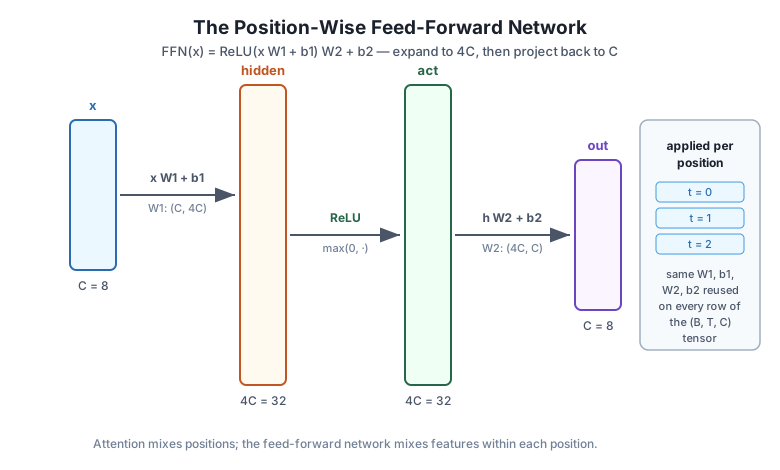
The idea is simple and the shapes are the whole story. Take the (B, T, C) tensor coming out of attention. For each position independently, run a tiny two-layer MLP: a linear layer that expands the width from C to 4C, a nonlinearity, and a second linear layer that projects back down to C. The same MLP is applied to every position, which is why it is called position-wise. Attention moves information between positions; the feed-forward network then lets each position chew on that information with real nonlinear capacity. The two alternate, block after block.

By the end of this lesson, you will be able to:

• Describe the feed-forward network as two linear layers with a nonlinearity between them, expanding to 4C and back to C
• Explain what “position-wise” means and why the FFN mixes features while attention mixes positions
• Explain why the nonlinearity is essential (two linear layers with nothing between them collapse into one)
• Implement ffn_forward with caching and ffn_backward in NumPy
• Verify every gradient (dW1, db1, dW2, db2, dx) against a float64 numerical gradient

You should be comfortable with the backward pass of a small MLP and with the (B, T, C) shape convention from earlier modules. Let’s begin.

What the Feed-Forward Network Computes#

The whole network is one formula. For an input x, the feed-forward network is

with two weight matrices and two bias vectors. The first linear layer uses $W_1$ of shape (C, 4C) and bias $b_1$ of length 4C; it takes a vector of width C up to a hidden width of 4C. The activation (we use ReLU) acts element-wise on those 4C numbers. The second linear layer uses $W_2$ of shape (4C, C) and bias $b_2$ of length C; it brings the hidden width back down to C, so the output has exactly the same shape as the input.

That expand-then-contract shape is deliberate. The hidden layer is conventionally four times wider than the model, and that wide middle is where the per-position computation happens. Widening to 4C gives the network a large, nonlinear intermediate space to combine and reshape the features it received from attention; projecting back to C keeps the block’s input and output shapes identical so blocks can be stacked without any glue. A transformer with model width C = 64 therefore has a feed-forward hidden width of 256.

The key structural fact is that this MLP has no notion of sequence position. It takes a single vector of width C and returns a single vector of width C. When we apply it to a (B, T, C) tensor, NumPy’s matrix multiply runs it on all B * T vectors at once, but each of those vectors is transformed completely independently of the others. Nothing in the feed-forward network lets position 5 see position 3. That separation of duties is the design: attention (and only attention) moves information between positions; the feed-forward network transforms each position on its own.

Why the Nonlinearity Is Essential#

It is tempting to think the two linear layers already give the network depth. They do not, and the reason is worth seeing clearly. Suppose you removed the activation, so the feed-forward network were just x W1 + b1 followed by ... W2 + b2. Ignoring biases for a moment, the composition is

and $W_1 W_2$ is itself a single (C, C) matrix. Two stacked linear layers with nothing between them are exactly equivalent to one linear layer with weight $W_1 W_2$. All that expensive expansion to 4C and back would buy you nothing: the model could represent the same function with a single (C, C) matrix. Depth without a nonlinearity is an illusion.

The activation breaks that collapse. ReLU, $\text{ReLU}(z) = \max(0, z)$, zeroes out the negative entries of the hidden vector, which is a genuinely nonlinear operation that no single matrix can reproduce. That one bend in the function is what lets the two-layer network represent things a single linear layer cannot. We use ReLU here because its gradient is clean and exact: it is 1 where the pre-activation was positive and 0 elsewhere. Real transformers often use GELU, a smooth cousin of ReLU defined as $\text{GELU}(z) = z \cdot \Phi(z)$ where $\Phi$ is the standard normal cumulative distribution function; it behaves like ReLU for large positive and negative inputs but curves gently through zero. Everything in this lesson works the same way with GELU swapped in; ReLU just makes the backward pass easier to check by hand.

We will confirm the collapse numerically at the end of the lesson, but the takeaway is already the important part: the nonlinearity is not a detail, it is the entire reason the feed-forward network is more than a single matrix.

The Forward Pass, With Caching#

Time to build it. We use a tiny configuration so a full finite-difference gradient check runs instantly, and float64 throughout so the check has the precision to trust. Take a batch of B = 2, sequence length T = 4, and model width C = 8, which makes the hidden width 4C = 32. Everything is seeded for reproducibility.

The forward pass computes the pre-activation h_pre = x @ W1 + b1, applies ReLU to get the hidden activation h, and projects back down to out = h @ W2 + b2. It returns a cache of the tensors the backward pass will need: the input x, the pre-activation h_pre (whose sign gates the ReLU gradient), the activation h (the input to the second linear layer), and the two weight matrices.

import numpy as np

np.random.seed(42)
B, T, C = 2, 4, 8      # batch, sequence length, model width
hidden = 4 * C         # 32: the FFN expands to 4*C then projects back

def relu(z):
    return np.maximum(z, 0)

def ffn_forward(x, W1, b1, W2, b2):
    # x: (B, T, C)
    h_pre = x @ W1 + b1       # (B, T, 4C)  first linear: expand to 4C
    h = relu(h_pre)           # (B, T, 4C)  nonlinearity
    out = h @ W2 + b2         # (B, T, C)   second linear: project back to C
    cache = (x, h_pre, h, W1, W2)
    return out, cache

# initialize inputs and parameters (float64 by default)
x  = np.random.randn(B, T, C)
W1 = np.random.randn(C, hidden) * 0.1
b1 = np.random.randn(hidden) * 0.1
W2 = np.random.randn(hidden, C) * 0.1
b2 = np.random.randn(C) * 0.1

out, cache = ffn_forward(x, W1, b1, W2, b2)
print("x shape      :", x.shape)
print("hidden shape :", cache[2].shape)
print("out shape    :", out.shape)

x shape      : (2, 4, 8)
hidden shape : (2, 4, 32)
out shape    : (2, 4, 8)

The shapes tell the whole story. The input is (2, 4, 8), the hidden activation swells to (2, 4, 32) in the middle, and the output comes back to (2, 4, 8), identical to the input. That shape preservation is exactly what lets a transformer stack this block as many times as it likes. Notice that x @ W1 works even though x is a 3-D tensor: NumPy treats the leading (B, T) axes as a batch and applies the (C, 4C) matrix multiply to each of the B * T position vectors, which is the position-wise behavior falling out for free.

The Backward Pass#

The feed-forward network is a standard two-layer MLP, so its backward pass is the standard MLP backprop you have seen before, now carrying the extra (B, T) batch axes. We receive dout, the gradient of the loss with respect to the output, and walk backward through the three operations in reverse order.

Through the second linear layer out = h @ W2 + b2. The weight gradient sums the outer product of the cached input h and the incoming gradient over every position in the batch, the bias gradient sums dout over the batch and sequence axes, and the gradient flows back to the hidden activation through $W_2^\top$:

Through the ReLU h = relu(h_pre). ReLU passes the gradient straight through wherever the pre-activation was positive and blocks it elsewhere, so we multiply dh by the cached mask (h_pre > 0):

Through the first linear layer h_pre = x @ W1 + b1. Same matrix-multiply rules as the second layer, with x now playing the role of the input, and the gradient continues back to the input x through $W_1^\top$:

The only new bookkeeping compared with a plain MLP is that the weight gradients must sum the per-position outer products over both the batch axis and the sequence axis. We use np.einsum('bti,btj->ij', ...) to do that contraction cleanly; it sums x[b,t] outer dh_pre[b,t] across all B * T positions, which is exactly the shared-weight gradient for a position-wise layer.

def ffn_backward(dout, cache):
    x, h_pre, h, W1, W2 = cache
    # second linear: out = h @ W2 + b2
    dW2 = np.einsum('bti,btj->ij', h, dout)   # (4C, C)
    db2 = dout.sum(axis=(0, 1))               # (C,)
    dh = dout @ W2.T                          # (B, T, 4C)
    # ReLU: h = relu(h_pre)
    dh_pre = dh * (h_pre > 0)                 # (B, T, 4C)
    # first linear: h_pre = x @ W1 + b1
    dW1 = np.einsum('bti,btj->ij', x, dh_pre) # (C, 4C)
    db1 = dh_pre.sum(axis=(0, 1))             # (4C,)
    dx = dh_pre @ W1.T                        # (B, T, C)
    return dx, dW1, db1, dW2, db2

# a fixed upstream gradient so the run is reproducible
np.random.seed(0)
dout = np.random.randn(*out.shape)           # dout = d(loss)/d(out)

dx, dW1, db1, dW2, db2 = ffn_backward(dout, cache)
print("dW1:", dW1.shape, "| db1:", db1.shape)
print("dW2:", dW2.shape, "| db2:", db2.shape)
print("dx :", dx.shape)

dW1: (8, 32) | db1: (32,)
dW2: (32, 8) | db2: (8,)
dx : (2, 4, 8)

Every gradient has exactly the same shape as the quantity it belongs to: dW1 matches W1 at (8, 32), dW2 matches W2 at (32, 8), the bias gradients match their biases, and dx matches the input x at (2, 4, 8). That shape-matching rule is the fastest sanity check you have; if any of these had failed to line up, there would be a missing transpose or a missing sum somewhere in the backward pass.

Proving It With a Gradient Check#

Shapes lining up means the code runs, not that it is correct. To prove the backward pass, we compare each analytic gradient against a numerical gradient: nudge one entry of a parameter by a tiny $\epsilon$, measure how the loss changes, and divide. By the definition of a derivative, the centered finite difference should match the analytic value:

We need a scalar loss for this. Any fixed scalar function of out works, so we use L = sum(out * G) for a fixed random tensor G; its gradient with respect to out is just G, which is the dout we already fed to the backward pass. We then sweep every entry of each parameter, compute the centered difference, and report the maximum relative error across all entries.

G = dout                                     # d(loss)/d(out) for L = sum(out * G)
def loss_of(x, W1, b1, W2, b2):
    return np.sum(ffn_forward(x, W1, b1, W2, b2)[0] * G)

def max_rel_err(analytic, param):
    eps = 1e-6
    worst = 0.0
    for idx in np.ndindex(*param.shape):
        orig = param[idx]
        param[idx] = orig + eps
        lp = loss_of(x, W1, b1, W2, b2)
        param[idx] = orig - eps
        lm = loss_of(x, W1, b1, W2, b2)
        param[idx] = orig                    # restore
        numeric = (lp - lm) / (2 * eps)
        denom = max(1e-12, abs(analytic[idx]) + abs(numeric))
        worst = max(worst, abs(analytic[idx] - numeric) / denom)
    return worst

print("max rel err dW1:", f"{max_rel_err(dW1, W1):.2e}")
print("max rel err db1:", f"{max_rel_err(db1, b1):.2e}")
print("max rel err dW2:", f"{max_rel_err(dW2, W2):.2e}")
print("max rel err db2:", f"{max_rel_err(db2, b2):.2e}")
print("max rel err dx :", f"{max_rel_err(dx, x):.2e}")

max rel err dW1: 1.29e-07
max rel err db1: 2.21e-09
max rel err dW2: 1.65e-08
max rel err db2: 2.71e-10
max rel err dx : 6.17e-08

Every relative error is on the order of 1e-7 or smaller, which is exactly what a correct backward pass produces in float64: the tiny residual is finite-difference truncation error, not a bug. The analytic gradients and the numerical gradients agree, so we can trust ffn_backward. Gradient checking is far too slow to run during training (it re-runs the forward pass twice per parameter entry), but it is the single most reliable way to catch a backward-pass mistake once, up front.

Seeing the Collapse#

One last check drives home why the nonlinearity matters. Earlier we argued that two linear layers with nothing between them are equivalent to a single linear layer, because $(x W_1) W_2 = x (W_1 W_2)$. Here it is in three lines: multiply through the two matrices in sequence, versus multiplying by their product, and confirm the results are identical.

np.random.seed(1)
A  = np.random.randn(C, hidden)      # stand-in for W1: (C, 4C)
Bm = np.random.randn(hidden, C)      # stand-in for W2: (4C, C)
xx = np.random.randn(5, C)

two_layers = (xx @ A) @ Bm           # two linear layers, no activation
one_layer  = xx @ (A @ Bm)           # a single (C, C) matrix
print("identical?", np.allclose(two_layers, one_layer))

identical? True

True. Without an activation, the expensive expansion to 4C and back is mathematically indistinguishable from one (C, C) matrix, so the model gains no representational power from the extra layer. Put the ReLU back between them and that equivalence breaks, which is precisely why the feed-forward network earns its place in the block.

Practice Exercises#

Try these before checking the hints. They reuse ffn_forward, ffn_backward, and the variables defined above.

Exercise 1: Swap in a Different Hidden Width#

Real transformers use a hidden width of 4C, but the code should work for any multiple. Rebuild W1, b1, W2, b2 with hidden = 2 * C instead, run the forward pass, and confirm the output is still (B, T, C) while the hidden activation is now (B, T, 2C).

# Your code here: set hidden = 2 * C, re-init the four parameters, run ffn_forward

Exercise 2: Gradient-Check a ReLU Boundary#

The ReLU gradient is 1 for positive pre-activations and 0 otherwise. Pick an entry of h_pre that is negative and confirm that increasing the corresponding W1 column has no effect on the loss through that unit, as long as the entry stays negative. What does that tell you about the gradient flowing into dW1 there?

# Your code here: find an index where h_pre < 0 and reason about its gradient

Exercise 3: Confirm Positions Are Independent#

The feed-forward network is position-wise, so changing one position’s input should never change another position’s output. Run the forward pass, then perturb x[0, 0] only, run again, and check that out[0, 1], out[0, 2], and out[0, 3] are unchanged while out[0, 0] moves.

# Your code here: perturb x[0, 0], re-run ffn_forward, compare the other positions

Summary#

You built the second half of the transformer block: the position-wise feed-forward network that gives each position its nonlinear computation. Let’s review.

Key Concepts#

The Big Idea

• The feed-forward network is a two-layer MLP applied independently to every position: $\text{FFN}(x) = \text{act}(x W_1 + b_1) W_2 + b_2$
• It expands the width from C to 4C, applies a nonlinearity, and projects back to C, so input and output shapes match and blocks can stack
• Attention mixes information across positions; the feed-forward network mixes features within each position. The two alternate

Why the Nonlinearity Matters

• Two linear layers with nothing between them collapse to one: $(x W_1) W_2 = x (W_1 W_2)$
• ReLU (or GELU) breaks that collapse and is the entire reason the FFN is more than a single matrix

The Backward Pass

• Second linear: dW2 = einsum('bti,btj->ij', h, dout), db2 = dout.sum((0,1)), dh = dout @ W2.T
• ReLU: dh_pre = dh * (h_pre > 0), gated by the cached sign
• First linear: dW1 = einsum('bti,btj->ij', x, dh_pre), db1 = dh_pre.sum((0,1)), dx = dh_pre @ W1.T
• Weight and bias gradients sum over all positions because the weights are shared across positions

Checking Your Work

• Every gradient has the same shape as its quantity
• A float64 numerical gradient check gave max relative errors near 1e-7 for dW1, db1, dW2, db2, and dx

Why This Matters#

The feed-forward network is where a large fraction of a transformer’s parameters and computation actually live. In a model with width C, the two feed-forward matrices hold roughly $2 \cdot C \cdot 4C = 8C^2$ parameters per block, typically more than the attention projections. When people talk about scaling a transformer’s capacity, they are very often talking about widening this hidden layer. Understanding it as a plain shared MLP, expand, activate, contract, demystifies a huge part of where a model’s knowledge is stored and how it is applied one position at a time.

It also completes the pair. You now have both halves of what happens inside a block: attention to route information between positions, and the feed-forward network to transform it at each position. Everything else in the block, the residual connections and the layer normalization from the earlier lessons in this module, exists to make a deep stack of these two operations trainable.

Continue Building Your Skills#

You have now built every ingredient of the transformer block in isolation: multi-head attention from Module 3, the residual connections and layer normalization from the first two lessons of this module, and now the position-wise feed-forward network. In the next lesson you assemble them into the complete pre-norm transformer block, the exact unit that a real transformer stacks over and over. You will wire attention and the feed-forward network together with layer norm applied before each and a residual connection wrapped around each, then run the whole block forward and backward and gradient-check it end to end. Once that block is verified and shape-preserving, stacking it into a deep network is just a loop, and the architecture you have been building piece by piece since Module 1 will finally be whole.