Lesson 4 - Assembling the Block

Welcome to Assembling the Block#

Over the last three lessons you built the parts that surround attention. You added residual connections so gradients survive depth, layer normalization to keep each position’s activations well-scaled, and the position-wise feed-forward network that gives every position room to compute. In Module 3 you built the other half: multi-head attention, the layer that lets positions share information. This lesson snaps all of it together into the single repeatable unit that a transformer is made of, the transformer block. Once you have one block that takes a (B, T, C) tensor and returns a (B, T, C) tensor, a deep transformer is just that block, stacked. Your mini-GPT will stack two of them; a large model stacks dozens.

The arrangement matters as much as the parts. Modern GPT-style models use the pre-norm layout, where layer normalization is applied before each sublayer, tucked inside the residual connection. You will see exactly why that ordering makes deep stacks trainable, implement transformer_block_forward in pure NumPy, watch the shape at every sub-step, and then stack blocks to prove the one structural property that makes the whole architecture possible: a block’s output is a valid input to the next block. This lesson is forward-only; the block’s backward pass is the guided project in Lesson 5.

By the end of this lesson, you will be able to:

• Write the two update equations of a pre-norm transformer block and name each piece
• Explain why layer norm goes before each sublayer (pre-norm) and why that beats putting it after (post-norm) for deep stacks
• Describe how each sublayer is wrapped in a residual connection and normalized on the way in
• Implement transformer_block_forward in NumPy from multi-head attention, two layer norms, the feed-forward network, and two residual adds
• Show that the block maps (B, T, C) to (B, T, C), and use that shape-preserving property to stack blocks

You should be comfortable with the residual, layer-norm, and feed-forward pieces from Lessons 1 to 3, and with multi_head_attention_forward from Module 3. Let’s assemble the block.

Two Sublayers, Each in a Residual#

A transformer block does two things in sequence. First it lets positions communicate through multi-head attention. Then it lets each position compute on its own through the feed-forward network. Each of those two operations is called a sublayer, and the block’s design rule is simple and uniform: every sublayer is wrapped in a residual connection, and normalized on the way in.

In the pre-norm layout, the whole block is just these two lines:

Read the first line from the inside out. Start with the block input $x$. Normalize it with the first layer norm. Feed that normalized copy into multi-head attention. Then add the result back to the original $x$. That addition is the residual connection: the sublayer never replaces $x$, it only computes a correction that gets added on. The second line does the identical dance with a second layer norm and the feed-forward network. Two sublayers, two layer norms, two residual adds, and the block is done.

Two details are worth stating precisely. First, each layer norm has its own learnable scale and shift ($\gamma$ and $\beta$); LayerNorm1 and LayerNorm2 are separate layers with separate parameters, not the same one reused. Second, the thing that gets added back in the residual is always the value from before that sublayer’s normalization, the raw $x$, not the normalized copy. The normalized tensor is only ever an input to the sublayer; it is never what flows down the residual highway.

Pre-Norm vs Post-Norm#

Where you place the layer norm turns out to be one of the most consequential design choices in the block, so it is worth slowing down on. There are two options.

The post-norm layout, from the original 2017 transformer, normalizes after the residual add:

The pre-norm layout, used by essentially every modern GPT, normalizes before the sublayer, inside the residual:

The difference looks small, but its effect on deep networks is large. In pre-norm, follow the residual path: the raw $x$ is added straight through, and the only thing between the block’s input and its output on that path is an addition. Nothing rescales $x$ as it travels down the stack. That gives gradients a clean, unobstructed highway from the loss all the way back to the earliest layers, which is exactly the property residual connections were invented to provide, now preserved no matter how many blocks you stack.

In post-norm, by contrast, every block ends by passing the summed result through a layer norm, so the residual signal is rescaled at every layer on its way back. Across dozens of blocks those rescalings compound, and the gradient path is no longer clean. Post-norm transformers are famously touchy to train deep, they typically need a careful learning-rate warmup and sometimes still diverge, whereas pre-norm stacks train stably out of the box. That reliability is why the field moved to pre-norm, and it is the layout you will build here.

One practical footnote: pre-norm leaves the very last block’s output un-normalized (the final residual add is the last thing that happens). Real models therefore add a single final layer norm after the last block, right before the output projection. Your mini-GPT will do the same in a later module; the block itself stays pure pre-norm.

The Block Preserves Shape#

Before writing the code, notice the single structural fact that everything depends on: the block does not change the shape of its input. Trace it. The input $x$ is (B, T, C). Layer norm normalizes along the last axis and returns (B, T, C). Multi-head attention, as you proved in Module 3, is shape-preserving: (B, T, C) in, (B, T, C) out. The residual add is elementwise, so it stays (B, T, C). The feed-forward network expands the width to $4C$ internally but contracts it right back to $C$, so it too returns (B, T, C). The final residual add is again elementwise. Every step preserves (B, T, C), so the block as a whole maps (B, T, C) to (B, T, C).

That is not a minor bookkeeping detail; it is the property that makes deep transformers possible. Because the output of a block has the exact same shape as its input, the output of one block is a valid input to the next block. You can therefore stack blocks like identical LEGO bricks, feeding each one’s output into the next, and the shapes always line up. A 2-block mini-GPT and a 96-block giant use the identical block definition; only the number of times you apply it changes. If the block reshaped its input, this would fall apart and you could not stack at all.

Implementing the Block#

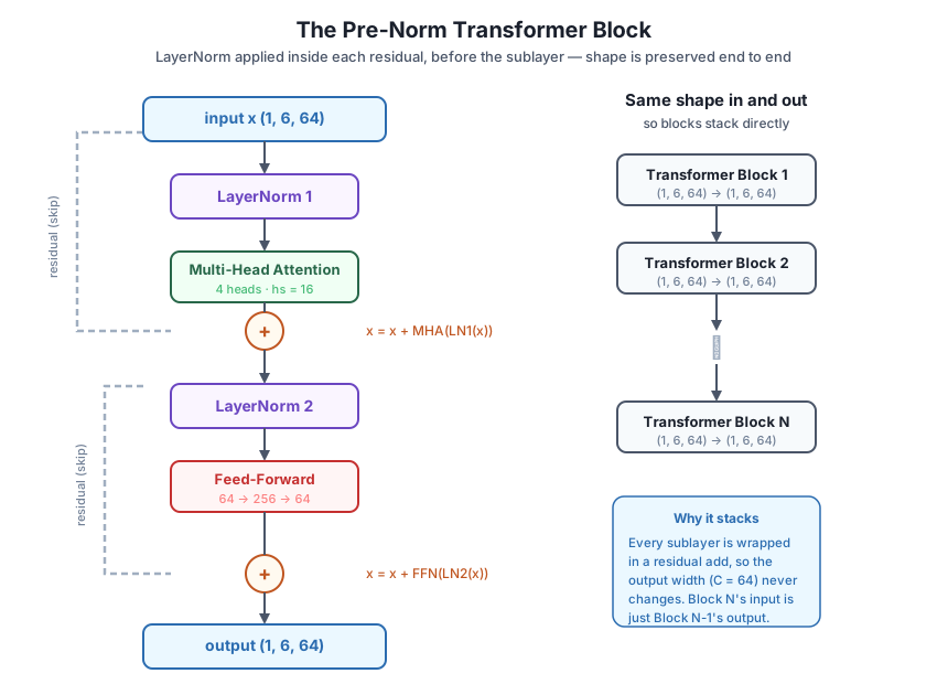
Here are the pieces, then the block. The multi-head attention forward is the exact function from Module 3. The layer norm normalizes along the last axis (the width $C$) and applies a per-feature scale $\gamma$ and shift $\beta$. The feed-forward network is the position-wise MLP from Lesson 3: a linear map that expands $C$ to $4C$, a GELU nonlinearity, and a linear map back to $C$.

import numpy as np

def softmax(x, axis=-1):
    x = x - x.max(axis=axis, keepdims=True)   # subtract row max for stability
    e = np.exp(x)
    return e / e.sum(axis=axis, keepdims=True)

def multi_head_attention_forward(X, Wq, Wk, Wv, Wo, h):
    B, T, C = X.shape
    hs = C // h
    Q = (X @ Wq).reshape(B, T, h, hs).transpose(0, 2, 1, 3)
    K = (X @ Wk).reshape(B, T, h, hs).transpose(0, 2, 1, 3)
    V = (X @ Wv).reshape(B, T, h, hs).transpose(0, 2, 1, 3)
    scores = Q @ K.transpose(0, 1, 3, 2) / np.sqrt(hs)   # (B, h, T, T)
    weights = softmax(scores, axis=-1)
    per_head = weights @ V                                # (B, h, T, hs)
    concat = per_head.transpose(0, 2, 1, 3).reshape(B, T, C)
    return concat @ Wo                                    # (B, T, C)

def layer_norm(x, gamma, beta, eps=1e-5):
    mu  = x.mean(axis=-1, keepdims=True)                  # per-position mean over C
    var = x.var(axis=-1, keepdims=True)                   # per-position variance over C
    xhat = (x - mu) / np.sqrt(var + eps)                  # standardize the last axis
    return gamma * xhat + beta                            # learned scale and shift

def gelu(x):
    return 0.5 * x * (1.0 + np.tanh(np.sqrt(2.0 / np.pi) * (x + 0.044715 * x**3)))

def feed_forward(x, W1, b1, W2, b2):
    hidden = gelu(x @ W1 + b1)                            # expand C -> 4C, nonlinearity
    return hidden @ W2 + b2                               # contract 4C -> C

Now the block itself. It takes the input x and a params dictionary holding every weight the block owns: the four attention projections, two independent pairs of layer-norm parameters, the two feed-forward weight matrices and biases, and the head count h. It applies the two pre-norm update equations exactly as written above, and returns the output. The verbose flag prints the shape at each sub-step so you can watch (B, T, C) survive the whole way through.

def transformer_block_forward(x, p, verbose=False):
    # --- Sublayer 1: multi-head attention, pre-norm, wrapped in a residual ---
    ln1  = layer_norm(x, p["ln1_gamma"], p["ln1_beta"])            # normalize on the way in
    attn = multi_head_attention_forward(ln1, p["Wq"], p["Wk"],
                                        p["Wv"], p["Wo"], p["h"])
    x    = x + attn                                                # residual add 1

    # --- Sublayer 2: feed-forward network, pre-norm, wrapped in a residual ---
    ln2  = layer_norm(x, p["ln2_gamma"], p["ln2_beta"])           # normalize on the way in
    ff   = feed_forward(ln2, p["W1"], p["b1"], p["W2"], p["b2"])
    out  = x + ff                                                  # residual add 2

    if verbose:
        print("LN1 out           :", ln1.shape,  "(B, T, C)")
        print("attention out     :", attn.shape, "(B, T, C)")
        print("after residual 1  :", x.shape,    "(B, T, C)")
        print("LN2 out           :", ln2.shape,  "(B, T, C)")
        print("FFN out           :", ff.shape,   "(B, T, C)")
        print("after residual 2  :", out.shape,  "(B, T, C)")
    return out

The body is a direct transcription of the two equations, with the x + ... on each line being the residual and the layer_norm(x, ...) inside each sublayer being the pre-norm. Notice that x after the first residual add is what feeds the second layer norm, exactly as the equations chain.

We need one helper to build a fresh block’s parameters. We seed with default_rng(42) for reproducibility and use the small 0.02 init that real transformers use (this lesson inspects shapes, not attention patterns, so the small training-scale init is the right choice). Layer norm starts at the identity, $\gamma = 1$ and $\beta = 0$, and biases start at zero.

def make_block_params(rng, C, h):
    return dict(
        Wq=rng.standard_normal((C, C)) * 0.02,
        Wk=rng.standard_normal((C, C)) * 0.02,
        Wv=rng.standard_normal((C, C)) * 0.02,
        Wo=rng.standard_normal((C, C)) * 0.02,
        ln1_gamma=np.ones(C),  ln1_beta=np.zeros(C),   # LN1 has its own gamma/beta
        ln2_gamma=np.ones(C),  ln2_beta=np.zeros(C),   # LN2 has its own gamma/beta
        W1=rng.standard_normal((C, 4 * C)) * 0.02,  b1=np.zeros(4 * C),
        W2=rng.standard_normal((4 * C, C)) * 0.02,  b2=np.zeros(C),
        h=h,
    )

Running One Block#

Time to run it. We use the mini-GPT width $C = 64$ with $h = 4$ heads (so $hs = 16$), on a single sequence of six tokens, $B = 1$, $T = 6$. The demo prints the shape at every sub-step and confirms the final output is (1, 6, 64), the same shape as the input.

rng = np.random.default_rng(42)
B, T, C, h = 1, 6, 64, 4
x = rng.standard_normal((B, T, C))
params = make_block_params(rng, C, h)

print("config: B=%d, T=%d, C=%d, h=%d, hs=%d" % (B, T, C, h, C // h))
print("input x           :", x.shape, "(B, T, C)")
print("-" * 40)
y = transformer_block_forward(x, params, verbose=True)
print("-" * 40)
print("final block output:", y.shape)
print("shape preserved (in == out)?", x.shape == y.shape)

config: B=1, T=6, C=64, h=4, hs=16
input x           : (1, 6, 64) (B, T, C)
----------------------------------------
LN1 out           : (1, 6, 64) (B, T, C)
attention out     : (1, 6, 64) (B, T, C)
after residual 1  : (1, 6, 64) (B, T, C)
LN2 out           : (1, 6, 64) (B, T, C)
FFN out           : (1, 6, 64) (B, T, C)
after residual 2  : (1, 6, 64) (B, T, C)
----------------------------------------
final block output: (1, 6, 64)
shape preserved (in == out)? True

Every single line reads (1, 6, 64). Layer norm, attention, the residual add, layer norm again, the feed-forward network, and the final residual add all hand back the exact shape they received. The feed-forward network expanded to 256 units internally, but the block’s interface never widened past 64. The block took a (1, 6, 64) tensor and returned a (1, 6, 64) tensor, which is the whole promise of the design.

Stacking Blocks#

Now the payoff. Because a block’s output shape matches its input shape, you can feed one block’s output straight into another. Give each block its own independent parameters (a real transformer never shares weights across blocks) and chain them. Here we stack two blocks, exactly as your mini-GPT will with n_layer = 2.

params_a = make_block_params(rng, C, h)   # block 1 gets its own weights
params_b = make_block_params(rng, C, h)   # block 2 gets its own weights

h1 = transformer_block_forward(x,  params_a)   # x  -> block 1
h2 = transformer_block_forward(h1, params_b)   # h1 -> block 2

print("input        :", x.shape)
print("after block 1:", h1.shape)
print("after block 2:", h2.shape)
print("two-block output still (1, 6, 64)?", h2.shape == (1, 6, 64))
print("sample out[0,0,:4]:", np.round(h2[0, 0, :4], 4))

input        : (1, 6, 64)
after block 1: (1, 6, 64)
after block 2: (1, 6, 64)
two-block output still (1, 6, 64)? True
sample out[0,0,:4]: [ 0.3635 -1.0432  0.7447  0.9527]

Block 1 turned x into h1, still (1, 6, 64); block 2 consumed h1 and produced h2, still (1, 6, 64). No reshaping, no adapter, no special first or last block, just the same function applied twice. That is a two-layer transformer’s forward pass in two lines.

To make the point unmistakable, stack six blocks in a loop and watch both the shape and the activation magnitude. If the shape-preserving property held only by luck, a deep stack would drift; instead every block hands back (1, 6, 64), and because pre-norm keeps the residual highway clean, the root-mean-square activation stays controlled from top to bottom rather than exploding or collapsing.

n_layer = 6
blocks = [make_block_params(rng, C, h) for _ in range(n_layer)]

hcur = x
print("start   :", hcur.shape, " RMS=%.4f" % np.sqrt((hcur**2).mean()))
for i, p in enumerate(blocks):
    hcur = transformer_block_forward(hcur, p)
    print("block %d :" % (i + 1), hcur.shape, " RMS=%.4f" % np.sqrt((hcur**2).mean()))
print("all shapes identical to input?", hcur.shape == x.shape)

start   : (1, 6, 64)  RMS=0.9526
block 1 : (1, 6, 64)  RMS=0.9530
block 2 : (1, 6, 64)  RMS=0.9522
block 3 : (1, 6, 64)  RMS=0.9522
block 4 : (1, 6, 64)  RMS=0.9507
block 5 : (1, 6, 64)  RMS=0.9519
block 6 : (1, 6, 64)  RMS=0.9522
all shapes identical to input?  True

Six blocks, six identical shapes, and an activation scale that barely moves from 0.95 across the whole depth. This is the structural guarantee that lets you write for block in blocks: x = block(x) and trust it to work at any depth. A production GPT is this exact loop run 12, 48, or 96 times. Every code block above is fully seeded; run any of them a second time and you get byte-for-byte identical numbers, including the 0.3635, -1.0432, 0.7447, 0.9527 sample.

Practice Exercises#

Try these before checking the hints. They reuse transformer_block_forward, make_block_params, the helper functions, and the seed-42 setup from the lesson.

Exercise 1: Build a Post-Norm Block and Compare#

Write a post_norm_block_forward(x, p) that uses the post-norm equations, x = LayerNorm1(x + MultiHeadAttention(x)) then x = LayerNorm2(x + FeedForward(x)), so the norm is applied after each residual add instead of before. Run it on the same x and confirm it still returns (1, 6, 64), then note that its output differs from the pre-norm block’s.

# Your code here: define post_norm_block_forward and run it on x

Exercise 2: Zero the Sublayers and Recover the Identity#

Set every attention and feed-forward weight in a block’s params to zero (leave the layer-norm gamma/beta alone) and run the block. Predict what the output should equal before you run it, then confirm.

# Your code here: zero Wq, Wk, Wv, Wo, W1, b1, W2, b2 in a params copy, run the block

Exercise 3: Stack N Blocks in a Function#

Write stack_forward(x, list_of_params) that applies a list of block parameter dicts in order and returns the final output. Use it to run a 4-block stack and confirm the output is (1, 6, 64). This is the core loop of a full transformer.

# Your code here: define stack_forward and run it on a list of 4 param dicts

Summary#

You assembled the full transformer block by combining multi-head attention, two layer norms, the feed-forward network, and two residual adds in the pre-norm order, and you proved it preserves shape so it can be stacked. Let’s review.

Key Concepts#

The Pre-Norm Block

• Two sublayers: x = x + MultiHeadAttention(LayerNorm1(x)) then x = x + FeedForward(LayerNorm2(x))
• Each sublayer is normalized on the way in and wrapped in a residual that adds the raw x back; the sublayer computes only a correction
• LayerNorm1 and LayerNorm2 are separate layers with their own gamma and beta

Pre-Norm vs Post-Norm

• Pre-norm normalizes the input to each sublayer and leaves the residual highway un-rescaled: x + Sub(LN(x))
• Post-norm normalizes the sum after each residual: LN(x + Sub(x)), which rescales the highway at every layer and compounds over depth
• Pre-norm gives gradients a clean path back and trains stably deep, which is why modern GPTs use it (a single final layer norm is added after the last block)

Shape Preservation

• Layer norm, attention, the residual add, and the feed-forward network each map (B, T, C) to (B, T, C), so the whole block does too
• The feed-forward network expands to $4C$ internally but contracts back to $C$, so the block’s interface width never changes

Stacking

• Because output shape equals input shape, one block’s output is a valid input to the next, so blocks stack with no adapters
• Stacking shares the block definition but gives each block its own parameters
• Demo (seed 42, B=1, T=6, C=64, h=4): one block, two stacked blocks, and six stacked blocks all returned (1, 6, 64), with the activation RMS holding near 0.95 across depth

Why This Matters#

The transformer block is the unit the entire architecture is built from, and you have now assembled one from parts you understand individually. The two ideas that make it work are worth carrying forward. The first is that arrangement is architecture: the same components in post-norm order give a network that is hard to train deep, while in pre-norm order they give one that trains stably to dozens of layers. When you read that a model is “pre-LN,” you now know it means the layer norm sits inside each residual, before the sublayer, and you know why that choice was made. The second is that shape preservation is what makes depth cheap: because a block is a (B, T, C) to (B, T, C) function, scaling a transformer up is literally a matter of applying the same function more times in a loop. There is no architectural difference between your 2-block mini-GPT and a 96-block frontier model, only the length of that loop and the size of $C$.

That uniformity is also what will make the backward pass tractable. A gradient has the same shape as the thing it belongs to, so once the forward shapes are second nature, backpropagating through the block is a matter of routing gradients through the same residual adds, layer norms, and attention in reverse, reusing the sublayer backward passes you already derived. That is exactly what the guided project builds next.

Continue Building Your Skills#

You can now assemble a complete pre-norm transformer block from multi-head attention, two layer norms, the feed-forward network, and two residual adds, and you have seen that its shape-preserving design is precisely what lets you stack blocks into a deep network. So far everything has flowed forward. The next lesson is the module’s guided project: you will package this block into a clean, reusable TransformerBlock class with a forward that caches its intermediates and a backward that routes the gradient back through both residual adds, both layer norms (reusing the subtle layer-norm backward you derived earlier), the feed-forward network, and multi-head attention, naming the attention gradients dQuery, dKey, and dValue to keep them distinct and deploy-safe. You will gradient-check the whole block against a numerical gradient, so that by the end you can trust every number your transformer block produces in both directions, ready to stack into the full mini-GPT in the modules ahead.