Lesson 5 - Guided Project: A Transformer Block Class

Welcome to the Guided Project#

Across this module you built the three things that turn attention into a deep, trainable network. Residual connections gave gradients a direct path backward, so depth stopped killing them. Layer normalization kept each position’s activations well-scaled from block to block, and you derived its subtle backward pass. The position-wise feed-forward network gave every token room to compute. And in Module 3 you packaged multi-head attention into its own gradient-checked class. In this guided project you stop treating those four pieces as loose code and assemble them into one object: a TransformerBlock class with a forward and a backward method, holding all of its own parameters and their gradients.

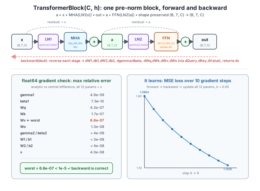
This is the unit of a transformer. A GPT is nothing more than this block stacked n_layer times, so getting it clean and provably correct now means Modules 6 and 7 inherit a component they can trust without re-deriving a single gradient. The block you build here is a pre-norm block: it normalizes before each sublayer and adds the result back to the input, the arrangement out = a + FFN(LN2(a)) where a = x + MHA(LN1(x)). That ordering is what lets you eventually stack a dozen of these and still train them. As always, the project ends the only way a serious layer should: a float64 gradient check against finite differences, and a short gradient-descent run that drives a real loss down.

By the end of this project, you will be able to:

• Structure a transformer block as a class that owns LayerNorm, multi-head attention, and feed-forward parameters plus their gradients
• Implement a pre-norm forward(x) that computes x + MHA(LN1(x)) then a + FFN(LN2(a)) and caches every value backward needs
• Implement backward(dout) so it flows gradients through both residual sublayers in reverse, accumulating grads for all twelve parameters and returning dx
• Gradient-check the entire block in float64, reporting the single worst relative error across every parameter and the input
• Run gradient-descent steps on the block and confirm a scalar loss decreases

This project assumes you followed the earlier lessons in this module (residuals, layer norm and its backward pass, the feed-forward network) and the multi-head attention class from Module 3. You only need numpy (version 2.x is fine) — no PyTorch, no GPU, no API key.

Stage 1: The Class#

A block owns four sub-components, and each contributes its own parameters. We set them all up in __init__, seeded so the class is reproducible, along with the two numbers that define its shape: the model width C and the number of heads h.

Counting the parameters keeps the design honest. LayerNorm1 contributes a scale gamma1 and shift beta1, each of length C. Multi-head attention contributes the four (C, C) matrices Wq, Wk, Wv, Wo you built in Module 3. LayerNorm2 adds another gamma2, beta2. And the feed-forward network — a two-layer MLP that expands to a hidden width of 4C and back — contributes W1 of shape (C, 4C), its bias b1, W2 of shape (4C, C), and b2. Twelve parameter arrays in all. The layer-norm scales start at one and the shifts at zero (the standard identity init), and every weight matrix is drawn small at * 0.02.

import numpy as np

def softmax(x, axis=-1):
    x = x - x.max(axis=axis, keepdims=True)   # stable: subtract row max
    e = np.exp(x)
    return e / e.sum(axis=axis, keepdims=True)

class TransformerBlock:
    """One pre-norm transformer block: LN1 -> MHA -> residual -> LN2 -> FFN -> residual."""

    def __init__(self, C, h, seed=42, eps=1e-5):
        assert C % h == 0, "C must be divisible by h"
        self.C, self.h, self.hs, self.eps = C, h, C // h, eps
        rng = np.random.default_rng(seed)
        # LayerNorm 1
        self.gamma1 = np.ones(C)
        self.beta1 = np.zeros(C)
        # Multi-head attention (four (C, C) matrices, from Module 3)
        self.Wq = rng.standard_normal((C, C)) * 0.02
        self.Wk = rng.standard_normal((C, C)) * 0.02
        self.Wv = rng.standard_normal((C, C)) * 0.02
        self.Wo = rng.standard_normal((C, C)) * 0.02
        # LayerNorm 2
        self.gamma2 = np.ones(C)
        self.beta2 = np.zeros(C)
        # Feed-forward network (hidden width = 4C)
        self.W1 = rng.standard_normal((C, 4 * C)) * 0.02
        self.b1 = np.zeros(4 * C)
        self.W2 = rng.standard_normal((4 * C, C)) * 0.02
        self.b2 = np.zeros(C)
        self.cache = None             # filled by forward, read by backward

block = TransformerBlock(C=8, h=4)
print("C, h, hs:", block.C, block.h, block.hs)
print("gamma1/beta1:", block.gamma1.shape, block.beta1.shape)
print("Wq/Wk/Wv/Wo:", block.Wq.shape, block.Wk.shape, block.Wv.shape, block.Wo.shape)
print("gamma2/beta2:", block.gamma2.shape, block.beta2.shape)
print("W1/b1:", block.W1.shape, block.b1.shape)
print("W2/b2:", block.W2.shape, block.b2.shape)
print("cache:", block.cache)

C, h, hs: 8 4 2
gamma1/beta1: (8,) (8,)
Wq/Wk/Wv/Wo: (8, 8) (8, 8) (8, 8) (8, 8)
gamma2/beta2: (8,) (8,)
W1/b1: (8, 32) (32,)
W2/b2: (32, 8) (8,)
cache: None

The skeleton holds exactly what the block must remember: its shape (C = 8, h = 4, so hs = 2), the twelve parameter arrays, and an empty cache slot. Notice that __init__ takes only C and h — the batch size B and sequence length T are never baked in, so the same object works on a (2, 6, 8) input today and a (32, 32, 64) input when we scale up in Module 7. The feed-forward hidden width is 4C = 32, which is why W1 is (8, 32) and W2 is (32, 8): expand to four times the width, apply a nonlinearity, contract back. That 4x expansion is the standard transformer ratio.

Stage 2: The forward Method#

Now we give the block a forward(x) method that runs the two pre-norm sublayers in order and — crucially — caches every value the backward pass will need. The structure is two residual stages stacked back to back:

Read it as two copies of the same pattern: normalize, run a sublayer, add the result back to what you started with. The first sublayer mixes information across positions (attention); the second transforms each position independently (the feed-forward network). Both are wrapped in a residual + so the untouched input always has a direct path to the output.

To keep the block self-contained, forward calls small helper methods for each piece — _ln_forward, _mha_forward, _ffn_forward — each of which returns its output and a per-sublayer cache. These are the exact forward passes you built earlier in this module and in Module 3, just gathered onto one object. The block-level cache is simply the four sub-caches bundled together.

class TransformerBlock:
    # ... __init__ from Stage 1 ...

    # ---- LayerNorm (normalizes over the last axis, width C) ----
    def _ln_forward(self, x, gamma, beta):
        mu = x.mean(-1, keepdims=True)
        xc = x - mu
        var = (xc ** 2).mean(-1, keepdims=True)
        inv = 1.0 / np.sqrt(var + self.eps)
        xhat = xc * inv
        out = gamma * xhat + beta
        return out, (xhat, inv, gamma)

    # ---- Multi-head attention (Module 3) ----
    def _mha_forward(self, x):
        B, T, C = x.shape
        h, hs = self.h, self.hs
        Q, K, V = x @ self.Wq, x @ self.Wk, x @ self.Wv
        Qh = Q.reshape(B, T, h, hs).transpose(0, 2, 1, 3)     # (B, h, T, hs)
        Kh = K.reshape(B, T, h, hs).transpose(0, 2, 1, 3)
        Vh = V.reshape(B, T, h, hs).transpose(0, 2, 1, 3)
        scores = Qh @ Kh.transpose(0, 1, 3, 2) / np.sqrt(hs)   # (B, h, T, T)
        A = softmax(scores, axis=-1)
        Oh = A @ Vh                                            # (B, h, T, hs)
        concat = Oh.transpose(0, 2, 1, 3).reshape(B, T, C)     # (B, T, C)
        out = concat @ self.Wo
        return out, (x, Qh, Kh, Vh, A, concat)

    # ---- Feed-forward network (expand to 4C, ReLU, contract) ----
    def _ffn_forward(self, x):
        z = x @ self.W1 + self.b1          # (B, T, 4C)
        hrelu = np.maximum(z, 0.0)
        out = hrelu @ self.W2 + self.b2    # (B, T, C)
        return out, (x, z, hrelu)

    def forward(self, x):
        ln1, ln1c = self._ln_forward(x, self.gamma1, self.beta1)
        mha_out, mhac = self._mha_forward(ln1)
        a = x + mha_out                                   # residual 1
        ln2, ln2c = self._ln_forward(a, self.gamma2, self.beta2)
        ffn_out, ffnc = self._ffn_forward(ln2)
        out = a + ffn_out                                 # residual 2
        self.cache = (ln1c, mhac, ln2c, ffnc)
        return out

np.random.seed(42)
B, T, C, h = 2, 6, 8, 4
X = np.random.randn(B, T, C).astype(np.float64)          # (2, 6, 8)
block = TransformerBlock(C, h)
out = block.forward(X)
print("in :", X.shape)
print("out:", out.shape)
print("shape preserved:", X.shape == out.shape)

in : (2, 6, 8)
out: (2, 6, 8)
shape preserved: True

The block preserves shape: (B, T, C) in, (B, T, C) out. This is the property that makes stacking possible — the output of one block is a valid input to the next, so you can chain as many as you like without any reshaping in between. Every sublayer inside either mixes across positions or transforms each position, but none of them changes the tensor’s shape, and the two residual adds only work because the sublayer output matches the input it is added to. Bundle the four sub-caches into self.cache and the forward pass is done; the backward pass will unpack them in reverse.

Stage 3: The backward Method#

This is where the block earns its keep. backward(dout) takes the gradient of the loss with respect to the block’s output and walks it back through the two residual stages in the exact reverse order of forward, filling in a gradient for all twelve parameters and returning dx.

The key move is how a residual connection routes gradients. Because out = a + ffn_out, the output gradient dout flows to both addends unchanged: it becomes the incoming gradient for the feed-forward branch and part of the gradient for a. So we start da as a copy of dout, push dout through the FFN and LN2 to get another contribution to da, and add it on. The same thing happens one stage down: a = x + mha_out, so da splits to the attention branch and to dx. This “the skip adds a copy of the gradient through” behavior is precisely why residuals keep gradients healthy through depth.

Inside the attention branch we name the gradients of the queries, keys, and values dQuery, dKey, and dValue (per-head versions carry an H suffix). The weight gradients stay dWq, dWk, dWv. Reading top to bottom is reading the forward pass in reverse:

class TransformerBlock:
    # ... __init__, _ln_forward, _mha_forward, _ffn_forward, forward ...

    def _ln_backward(self, dout, cache):
        xhat, inv, gamma = cache
        C = dout.shape[-1]
        dgamma = (dout * xhat).sum(axis=(0, 1))
        dbeta = dout.sum(axis=(0, 1))
        dxhat = dout * gamma
        dx = (inv / C) * (C * dxhat
                          - dxhat.sum(-1, keepdims=True)
                          - xhat * (dxhat * xhat).sum(-1, keepdims=True))
        return dx, dgamma, dbeta

    def _mha_backward(self, dout, cache):
        x, Qh, Kh, Vh, A, concat = cache
        B, T, C = x.shape
        h, hs = self.h, self.hs
        dWo = np.einsum('btc,btd->cd', concat, dout)
        dconcat = dout @ self.Wo.T
        dOh = dconcat.reshape(B, T, h, hs).transpose(0, 2, 1, 3)
        dA = dOh @ Vh.transpose(0, 1, 3, 2)
        dValueH = A.transpose(0, 1, 3, 2) @ dOh
        dS = A * (dA - (dA * A).sum(axis=-1, keepdims=True))     # softmax backward
        dscores = dS / np.sqrt(hs)
        dQueryH = dscores @ Kh
        dKeyH = dscores.transpose(0, 1, 3, 2) @ Qh
        dQuery = dQueryH.transpose(0, 2, 1, 3).reshape(B, T, C)
        dKey = dKeyH.transpose(0, 2, 1, 3).reshape(B, T, C)
        dValue = dValueH.transpose(0, 2, 1, 3).reshape(B, T, C)
        dWq = np.einsum('btc,btd->cd', x, dQuery)
        dWk = np.einsum('btc,btd->cd', x, dKey)
        dWv = np.einsum('btc,btd->cd', x, dValue)
        dx = dQuery @ self.Wq.T + dKey @ self.Wk.T + dValue @ self.Wv.T
        return dx, dWq, dWk, dWv, dWo

    def _ffn_backward(self, dout, cache):
        x, z, hrelu = cache
        dW2 = np.einsum('btc,btd->cd', hrelu, dout)
        db2 = dout.sum(axis=(0, 1))
        dhrelu = dout @ self.W2.T
        dz = dhrelu * (z > 0)                                    # ReLU gate
        dW1 = np.einsum('btc,btd->cd', x, dz)
        db1 = dz.sum(axis=(0, 1))
        dx = dz @ self.W1.T
        return dx, dW1, db1, dW2, db2

    def backward(self, dout):
        ln1c, mhac, ln2c, ffnc = self.cache
        # out = a + ffn_out : gradient reaches BOTH addends
        da = dout.copy()
        dln2, self.dW1, self.db1, self.dW2, self.db2 = self._ffn_backward(dout, ffnc)
        d_a, self.dgamma2, self.dbeta2 = self._ln_backward(dln2, ln2c)
        da += d_a
        # a = x + mha_out : gradient reaches BOTH addends
        dx = da.copy()
        dln1, self.dWq, self.dWk, self.dWv, self.dWo = self._mha_backward(da, mhac)
        d_x, self.dgamma1, self.dbeta1 = self._ln_backward(dln1, ln1c)
        dx += d_x
        return dx

np.random.seed(42)
B, T, C, h = 2, 6, 8, 4
X = np.random.randn(B, T, C).astype(np.float64)
block = TransformerBlock(C, h)
out = block.forward(X)

dout = np.random.randn(*out.shape)            # a pretend gradient from above
dX = block.backward(dout)
print("dX          :", dX.shape)
print("dWq/dWo     :", block.dWq.shape, block.dWo.shape)
print("dW1/dW2     :", block.dW1.shape, block.dW2.shape)
print("dgamma1/dbeta2:", block.dgamma1.shape, block.dbeta2.shape)

dX          : (2, 6, 8)
dWq/dWo     : (8, 8) (8, 8)
dW1/dW2     : (8, 32) (32, 8)
dgamma1/dbeta2: (8,) (8,)

Every gradient has the same shape as the parameter it belongs to — the first sanity check, and it passes: dWq matches Wq at (8, 8), dW1 matches W1 at (8, 32), dgamma1 matches gamma1 at (8,), and dX matches the input at (2, 6, 8). Look closely at backward and you can see the residual doing its job twice: da = dout.copy() seeds the gradient of a with the undiminished output gradient, and then da += d_a adds the part that came back through the feed-forward sublayer. The same two lines repeat for the lower residual, seeding dx and then adding the attention branch’s contribution. That copy-and-add is the residual connection in the backward direction, and it is what a shape check cannot verify. Matching shapes is necessary but not sufficient; the next stage proves the numbers are right.

Stage 4: Verify the Block Is Correct#

A backward pass you cannot verify is a backward pass you cannot trust — and this one has twelve parameters and two residual sublayers, so there is plenty of room for a subtle sign error or a misrouted gradient. We prove it two ways: a gradient check (do the analytic gradients match finite differences?) and a learning check (does a real loss go down when we descend them?).

Gradient Check#

The idea is the definition of a derivative. Nudge one entry of a parameter by $\pm \epsilon$, measure how much a scalar loss changes, and divide — that finite difference must match the analytic gradient:

We use a scalar loss $L = \sum(\text{out} \odot G)$ for a fixed random matrix $G$ of shape (B, T, C), because then the analytic gradient flowing into backward is exactly dout = G. We run the check in float64 — finite differences are numerically delicate, and single precision would drown the signal in rounding noise. One subtlety: at the default * 0.02 init the attention weights come out nearly uniform, which makes some gradients shrink toward finite-difference noise and inflates their relative error even when they are correct. So for the check we reinitialize the weights at a moderate * 0.5 scale, giving every gradient real signal to compare against. We report the single worst relative error across all twelve parameters and the input x.

def scalar_loss(out, G):
    return np.sum(out * G)

def rel_err(a, b):
    return np.max(np.abs(a - b) / np.maximum(1e-12, np.abs(a) + np.abs(b)))

def numeric_grad(block, X, P, G, eps=1e-6):
    """Central-difference gradient of scalar_loss w.r.t. every entry of array P."""
    g = np.zeros_like(P)
    it = np.nditer(P, flags=['multi_index'])
    while not it.finished:
        idx = it.multi_index
        old = P[idx]
        P[idx] = old + eps; lp = scalar_loss(block.forward(X), G)
        P[idx] = old - eps; lm = scalar_loss(block.forward(X), G)
        P[idx] = old
        g[idx] = (lp - lm) / (2 * eps)
        it.iternext()
    return g

np.random.seed(42)
B, T, C, h = 2, 6, 8, 4
X = np.random.randn(B, T, C).astype(np.float64)
block = TransformerBlock(C, h)
# moderate init so every gradient carries real signal (see note above)
gc = np.random.default_rng(3)
block.Wq = gc.standard_normal((C, C)) * 0.5
block.Wk = gc.standard_normal((C, C)) * 0.5
block.Wv = gc.standard_normal((C, C)) * 0.5
block.Wo = gc.standard_normal((C, C)) * 0.5
block.W1 = gc.standard_normal((C, 4 * C)) * 0.5
block.W2 = gc.standard_normal((4 * C, C)) * 0.5
block.gamma1 = gc.standard_normal(C) * 0.5 + 1.0
block.gamma2 = gc.standard_normal(C) * 0.5 + 1.0
block.beta1 = gc.standard_normal(C) * 0.5
block.beta2 = gc.standard_normal(C) * 0.5
G = np.random.randn(B, T, C)                  # fixed upstream gradient

block.forward(X)
dX = block.backward(G)                         # analytic grads for all 12 params + dX

params = [("gamma1", block.gamma1, block.dgamma1), ("beta1", block.beta1, block.dbeta1),
          ("Wq", block.Wq, block.dWq), ("Wk", block.Wk, block.dWk),
          ("Wv", block.Wv, block.dWv), ("Wo", block.Wo, block.dWo),
          ("gamma2", block.gamma2, block.dgamma2), ("beta2", block.beta2, block.dbeta2),
          ("W1", block.W1, block.dW1), ("b1", block.b1, block.db1),
          ("W2", block.W2, block.dW2), ("b2", block.b2, block.db2)]

worst, worst_name = 0.0, None
for name, P, analytic in params:
    e = rel_err(analytic, numeric_grad(block, X, P, G))
    print(f"  {name:7s} {e:.3e}")
    if e > worst:
        worst, worst_name = e, name

block.forward(X); dX = block.backward(G)       # recompute analytic dX
eX = rel_err(dX, numeric_grad(block, X, X, G))
print(f"  {'x':7s} {eX:.3e}")
if eX > worst:
    worst, worst_name = eX, "x"
print("max rel err (worst):", f"{worst:.3e}", "on", worst_name)

  gamma1  4.917e-09
  beta1   7.478e-10
  Wq      4.266e-07
  Wk      1.748e-07
  Wv      6.628e-07
  Wo      1.301e-08
  gamma2  6.912e-10
  beta2   3.910e-09
  W1      2.446e-08
  b1      3.194e-09
  W2      3.609e-08
  b2      9.258e-10
  x       4.020e-08
max rel err (worst): 6.628e-07 on Wv

Every one of the thirteen relative errors is around $10^{-7}$ or far smaller — the worst, on Wv, is 6.6e-07, comfortably under the 1e-5 bar for “the backward pass is correct.” The pattern is telling: the layer-norm and bias gradients (gamma, beta, b1, b2) are the most accurate at 10^{-9} or 10^{-10} because they flow through the fewest operations, while Wq, Wk, Wv accumulate slightly more finite-difference noise because their gradients thread all the way back through the softmax in every head. All thirteen are tiny, which is the numerical proof that backward — both residuals, both layer norms, multi-head attention, and the feed-forward network — implements the true derivative of forward.

It Learns#

Matching finite differences proves the gradients are correct; the final check proves they are useful. We pick a fixed random target Y of shape (B, T, C), define a mean-squared-error loss between the block’s output and Y, and take ten gradient-descent steps — each a forward, a backward, and a subtraction of lr times every parameter gradient. We use a moderate init again so the output carries signal. If the gradients truly point downhill, the printed loss must fall.

np.random.seed(0)
B, T, C, h = 2, 6, 8, 4
X = np.random.randn(B, T, C)
Y = np.random.randn(B, T, C)                  # a fixed random target to fit

tb = TransformerBlock(C, h)
rng = np.random.default_rng(7)                # larger init so the output has signal
tb.Wq = rng.standard_normal((C, C)) * 0.3
tb.Wk = rng.standard_normal((C, C)) * 0.3
tb.Wv = rng.standard_normal((C, C)) * 0.3
tb.Wo = rng.standard_normal((C, C)) * 0.3
tb.W1 = rng.standard_normal((C, 4 * C)) * 0.3
tb.W2 = rng.standard_normal((4 * C, C)) * 0.3
lr = 0.05

updates = [("Wq", "dWq"), ("Wk", "dWk"), ("Wv", "dWv"), ("Wo", "dWo"),
           ("gamma1", "dgamma1"), ("beta1", "dbeta1"),
           ("gamma2", "dgamma2"), ("beta2", "dbeta2"),
           ("W1", "dW1"), ("b1", "db1"), ("W2", "dW2"), ("b2", "db2")]

for step in range(10):
    o = tb.forward(X)
    loss = 0.5 * np.mean((o - Y) ** 2)
    dout = (o - Y) / o.size                    # gradient of the MSE loss
    tb.backward(dout)
    for p, g in updates:
        setattr(tb, p, getattr(tb, p) - lr * getattr(tb, g))
    print(f"step {step:2d}  loss {loss:.4f}")

step  0  loss 1.5964
step  1  loss 1.5064
step  2  loss 1.4314
step  3  loss 1.3687
step  4  loss 1.3154
step  5  loss 1.2687
step  6  loss 1.2263
step  7  loss 1.1878
step  8  loss 1.1527
step  9  loss 1.1200

The loss falls monotonically from 1.5964 to 1.1200 across ten steps — every step lower than the last, no bump. That is the whole training loop of a real network in miniature: forward, compute a loss, backward, nudge all twelve parameters against their gradients, repeat. A single small block cannot perfectly fit a random target, so the loss keeps descending rather than snapping to zero, but the steady, gap-free descent is exactly what correct gradients produce. Run this whole stage a second time and, because every draw is seeded, you get byte-for-byte identical errors and losses — this course has no nondeterminism to hide behind.

Practice Exercises#

Try these before checking the hints. They reuse the TransformerBlock class and the setup you built above.

Exercise 1: Gradient-Check a Bigger Block#

Rerun the Stage 4 gradient check with a larger configuration — say B, T, C, h = 3, 5, 16, 8 (so hs = 2 and the feed-forward hidden width is 4C = 64). Confirm the worst relative error across all twelve parameters and x is still under 1e-5. A correct backward pass should not care about the sizes or the number of heads.

# Your code here: rebuild X, block, G with the larger shapes and re-run the check

Exercise 2: Show the Residuals Matter#

Temporarily remove the two residual connections — make forward compute a = mha_out (drop the x +) and out = ffn_out (drop the a +) — and rerun the “it learns” loop. Compare how far the loss falls in ten steps against the residual version’s 1.1200.

# Your code here: a forward without the two residual adds, then the Stage 4 loop

Exercise 3: Freeze the Feed-Forward Network#

In the “it learns” loop, stop updating the four feed-forward parameters (W1, b1, W2, b2) — keep updating attention and both layer norms. Does the loss still fall, and does it reach as low as 1.1200?

# Your code here: update every parameter EXCEPT W1, b1, W2, b2 each step

Summary#

You turned an entire module’s worth of pieces into one reusable, provably correct component — the exact unit a GPT stacks. Let’s review what you built.

Key Concepts#

The Class Design

• __init__(C, h) stores the shape (C, h, hs = C // h) and twelve parameter arrays: gamma1/beta1, the four attention matrices Wq/Wk/Wv/Wo, gamma2/beta2, and the feed-forward W1/b1/W2/b2 with hidden width 4C
• The block commits only to widths (C, h), never to B or T, so the same object works on any batch size or sequence length
• Parameters, a forward cache, and gradients all live on self

Pre-Norm forward and backward

• forward(x) computes a = x + MHA(LN1(x)) then out = a + FFN(LN2(a)), preserving the (B, T, C) shape so blocks stack cleanly, and caches every sublayer’s values
• backward(dout) reverses both residual stages: a residual + sends the gradient to both addends, so da (and later dx) is seeded with a copy of the incoming gradient and then accumulates the sublayer branch on top
• Inside attention the query/key/value gradients are dQuery, dKey, dValue; the weight gradients stay dWq, dWk, dWv

Proving Correctness

• A float64 central-difference gradient check gave a worst relative error of 6.6e-07 (on Wv), with layer-norm and bias grads down at 10^{-9} or smaller — all thirteen under the 1e-5 bar
• A ten-step gradient-descent run drove a real MSE loss monotonically from 1.5964 to 1.1200, confirming the gradients point downhill
• Everything is seeded and byte-for-byte reproducible on a second run

Why This Matters#

This class is the single most reused object in the whole course. A GPT is literally this block stacked n_layer times: the output of one block, still shape (B, T, C), is the input to the next, and that is only possible because you built the block to preserve shape and wrapped each sublayer in a residual so gradients survive the depth. Because you gradient-checked the entire block here — both layer norms, multi-head attention, the feed-forward network, and both residuals — Modules 6 and 7 inherit a component known to be correct and never have to re-derive a gradient.

More broadly, you have now seen the deepest instance of the forward-caches / backward-reads-the-cache pattern you will build before the full model: four sub-components, each with its own cache, composed into one object whose backward pass is just its sublayers’ backward passes run in reverse with residual adds threaded through. That compositional structure — small verified pieces assembled into a bigger verified piece — is exactly how real deep-learning libraries are built, and it is why you can trust a transformer you assembled yourself rather than treating it as a black box.

Continue Building Your Skills#

You now hold a single, trustworthy transformer block packaged as a class — the workhorse unit that the rest of the course simply repeats. But there is one thing it cannot yet do, and it is the thing that makes a language model: right now every position can attend to every other position, including ones in the future. A model that peeks ahead can trivially “predict” the next character by reading it, which teaches it nothing. In the next module, Causal Masking and the GPT, you will add a causal mask to the attention scores so position t can only attend to positions t and earlier, then stack several of these blocks into a real GPT and wire up the token and positional embeddings from Module 4 at its input. Keep this gradient-checked block close — the mask is a small change to one line of forward, and once it is in place, this exact class becomes the beating heart of a model that can actually generate text.