Lesson 2 - The Adam Optimizer

Welcome to The Adam Optimizer#

You have batches and you have a model that produces a loss and gradients. The last missing piece of a training step is the rule that turns those gradients into weight updates: the optimizer. Plain gradient descent — subtract a fixed multiple of the gradient — technically works, but for a model with hundreds of thousands of parameters spanning very different scales it is painfully slow and fragile. Transformers are trained with Adam, and in this lesson you’ll build it yourself and see exactly why it wins.

By the end of this lesson, you will be able to:

• Explain why one global learning rate struggles when parameters have different curvature
• State Adam’s update rule: first moment, second moment, and bias correction
• Implement an Adam optimizer class in NumPy that updates parameters in place
• Show, on an ill-conditioned problem, that Adam converges where SGD stalls

Why One Learning Rate Isn’t Enough#

Gradient descent updates every parameter with the same rule, $w \mathrel{-}= \text{lr} \cdot g$. The trouble is that the loss surface is not equally steep in every direction. If one parameter sits in a steep, high-curvature direction and another in a shallow one, a learning rate small enough to be stable in the steep direction is far too small to make progress in the shallow one. You end up crawling along the flat directions to avoid diverging along the steep ones.

Adam (Adaptive Moment Estimation) fixes this by giving every parameter its own effective step size, scaled down where gradients have been large and up where they’ve been small. It does this by tracking two running averages per parameter.

The first moment $m$ is a decaying average of the gradient (momentum — it smooths out noise):

The second moment $v$ is a decaying average of the squared gradient (a per-parameter scale estimate):

Both start at zero, which biases them toward zero on the early steps, so Adam bias-corrects them:

and finally takes the step, dividing the smoothed gradient by the square root of its typical size:

The defaults $\beta_1 = 0.9$, $\beta_2 = 0.999$, $\epsilon = 10^{-8}$ are used almost universally.

Implementing Adam#

Adam keeps one m and one v array per parameter tensor, plus a step counter t for the bias correction. Here it is in full — a class that updates a dictionary of parameters in place given a matching dictionary of gradients.

import numpy as np

class Adam:
    def __init__(self, params, lr=1e-3, beta1=0.9, beta2=0.999, eps=1e-8):
        self.lr, self.beta1, self.beta2, self.eps = lr, beta1, beta2, eps
        self.t = 0
        self.m = {k: np.zeros_like(v) for k, v in params.items()}
        self.v = {k: np.zeros_like(v) for k, v in params.items()}

    def step(self, params, grads):
        self.t += 1
        for k in params:
            g = grads[k]
            self.m[k] = self.beta1 * self.m[k] + (1 - self.beta1) * g
            self.v[k] = self.beta2 * self.v[k] + (1 - self.beta2) * (g * g)
            m_hat = self.m[k] / (1 - self.beta1 ** self.t)
            v_hat = self.v[k] / (1 - self.beta2 ** self.t)
            params[k] -= self.lr * m_hat / (np.sqrt(v_hat) + self.eps)

That’s the whole optimizer. The 1 - beta1 ** self.t and 1 - beta2 ** self.t terms are the bias correction: on step 1 they are 0.1 and 0.001, which rescale the near-zero raw moments up to sensible magnitudes so the very first update isn’t microscopic.

Adam vs. SGD on an Ill-Conditioned Problem#

To see the difference, we need a problem where curvature varies across directions. Take a quadratic bowl whose steepness differs by a factor of 1000 across its 20 dimensions:

The gradient is $2 c_i (w_i - t_i)$. The steep dimensions ($c_i = 1000$) force any stable SGD learning rate to be tiny, which starves the shallow dimensions ($c_i = 1$). Adam, adapting per parameter, sidesteps the whole problem.

rng = np.random.default_rng(42)
curv = np.geomspace(1, 1000, 20)      # condition number 1000
target = rng.normal(0, 1, 20)

def loss_and_grad(w):
    return float((curv * (w - target) ** 2).sum()), 2 * curv * (w - target)

# Adam
params = {"w": np.zeros(20)}
opt = Adam(params, lr=0.1)
print("Adam (lr=0.1):")
for step in range(200):
    loss, g = loss_and_grad(params["w"])
    opt.step(params, {"w": g})
    if step in (0, 5, 20, 50, 100, 199):
        print(f"  step {step:3d}  loss {loss:.4f}")

# SGD at its largest stable rate (bigger diverges on the c=1000 dimension)
w = np.zeros(20)
print("SGD (lr=0.001):")
for step in range(200):
    loss, g = loss_and_grad(w)
    if step in (0, 5, 20, 50, 100, 199):
        print(f"  step {step:3d}  loss {loss:.4f}")
    w -= 0.001 * g

Adam (lr=0.1):
  step   0  loss 1495.8765
  step   5  loss 319.6040
  step  20  loss 102.4265
  step  50  loss 2.5531
  step 100  loss 0.0189
  step 199  loss 0.0000
SGD (lr=0.001):
  step   0  loss 1495.8765
  step   5  loss 80.0909
  step  20  loss 29.2436
  step  50  loss 16.0918
  step 100  loss 8.5413
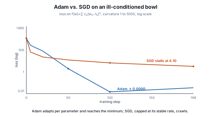
  step 199  loss 4.1042

Both start at the same loss of 1495.88. Adam drives it to essentially zero by step 100 and reaches the exact minimum by step 199. SGD, held to lr=0.001 (anything larger diverges along the steepest dimension), makes fast early progress on the steep directions but then stalls, still at loss 4.10 after 200 steps because it can barely move along the shallow ones. This gap — convergence versus a stall — is exactly why transformer training uses Adam. Both runs are fully reproducible from the fixed seed.

Practice Exercises#

Exercise 1: The effect of bias correction#

Print 1 - 0.9**t and 1 - 0.999**t for t = 1, 2, 10. Which moment (first or second) is corrected more aggressively on the first step, and why does that matter?

Exercise 2: SGD’s stability ceiling#

Re-run the SGD loop with lr=0.002 and then lr=0.01. At what point does the loss blow up instead of shrinking, and which dimension is responsible?

Exercise 3: Momentum only#

Modify step to skip the second-moment scaling (use params[k] -= lr * m_hat), turning Adam into plain momentum. Does it still stall on this problem like SGD?

Summary#

Adam gives every parameter its own adaptive step size by tracking a decaying average of the gradient (the first moment, for momentum) and of the squared gradient (the second moment, for per-parameter scale), bias-correcting both, and stepping by m_hat / (sqrt(v_hat) + eps). On an ill-conditioned problem it converges to the exact minimum while SGD, capped at its largest stable learning rate, stalls — the concrete reason Adam is the default optimizer for transformers.

Key Concepts#

• First moment m: decaying average of the gradient; momentum that smooths noise.
• Second moment v: decaying average of the squared gradient; a per-parameter scale estimate.
• Bias correction: dividing by 1 - beta**t to undo the zero-initialization bias on early steps.
• Adaptive step: m_hat / (sqrt(v_hat) + eps) is roughly unit-scale in every direction, regardless of curvature.

Why This Matters#

A transformer’s parameters — embeddings, attention projections, layer-norm scales, the output head — live at very different scales and see very differently sized gradients. A single global learning rate would force you to tune it for the touchiest tensor and starve all the others, which is why from-scratch training with plain SGD is so frustrating. Adam removes that tuning burden: with its default betas and one reasonable learning rate, it just works, which is why essentially every large language model is trained with it or a close variant. Building it yourself demystifies the one line, optimizer.step(), that every training loop leans on.

Continue Building Your Skills#

You now have both halves of a training step: batches from Lesson 1 and an optimizer that knows how to use gradients. The next lesson connects them to the model. You’ll write the training loop — sample a batch, run the forward pass to get the loss, run the backward pass to get the gradients, take an Adam step, and repeat — and run it for real on the mini-GPT, watching the loss fall from the random baseline of about 3.18 toward a model that has genuinely learned the Lantern Bay text.